Special Issue Article Open Access
Virtual Prototype Simulation of Truck Vibrations in High-Impact Shovel Loading Operations
Nassib Aouad1*and Samuel Frimpong21Assistant Professor of Mining Engineering, Missouri S&T, Rolla, MO, USA
2Robert Quenon Endowed Chair and Professor of Mining Engineering, Missouri S&T, Rolla, MO, USA
- *Corresponding Author:
- Nassib Aouad
Assistant Professor of Mining Engineering
Missouri S&T, Rolla, MO, USA
E-mail: narzf@mst.edu
Received Date: January 15, 2013; Accepted Date: January 17, 2013; Published Date: January 26, 2013
Citation: Aouad N, Frimpong S (2013) Virtual Prototype Simulation of Truck Vibrations in High-Impact Shovel Loading Operations. J Powder Metall Min S1:004. doi: 10.4172/2168-9806.S1-004
Copyright: © 2013 Aouad N, et al. This is an open-access article distributed under the terms of the Creative Commons Attribution License, which permits unrestricted use, distribution, and reproduction in any medium, provided the original author and source are credited.
Visit for more related articles at Journal of Powder Metallurgy & Mining
Abstract
Virtual prototyping has dramatically increased in the past decades due to powerful computing tools and environment. Moreover, companies are under pressure to reduce development and optimization time for their future products. With virtual prototyping, engineers can explore the performance and behavior of various design alternatives without investing time and money required to build actual prototypes. Also, in dangerous applications, human factor can be analyzed in a virtual prototype without compromising their health and safety. This paper highlights the development of a 3D virtual prototype simulator for truck vibrations under High-Impact Shovel Loading Operations (HISLO) conditions. It contains a complete methodology and procedure for building the complex dynamic model, with multi-degrees of freedom that best captures the actual truck under the HISLO conditions. The detailed steps and methodologies for building the virtual model using MSC.ADAMSare also discussed in this paper. The constraints, dimensions and control environments of this virtual model are described. This study also focuses on the methods used in MSC.ADAMSto build the complex dynamic model, and their limitations for developing and simulating the virtual prototype simulators.
Keywords
Virtual prototyping; HISLO; WBV; Truck vibrations; MSC.ADAMS; Dynamic modeling
Introduction
The deployment of large machinery for low cost, bulk surface mine production operations has resulted in High-Impact Shovel Loading Operations (HISLO). In extreme cases, shovels load large dump trucks with 100ton (or more) passes generating high-impact forces under gravity. HISLO generates high-frequency shockwaves that cause severe truck vibrations exposing operators to Whole Body Vibrations (WBV). These extreme conditions may limit operators’ performance and further impact the overall system performance. Furthermore, the WBV levels in such cases may exceed the recommended International Standards Organization (ISO) limits resulting in long-term lower-back disorders and other health problems. There is a need for fundamental and applied research to determine HISLO vibration levels, their comparisons to ISO 2631[1-4]limits and the safety of operators under these conditions. This paper pioneers in studying and analyzing this vibration problem using virtual prototyping techniques. The truck virtual prototype allows sever scenarios to be investigated efficiently and cut solution and optimization time period without abusing the machine and compromising operator’s health and safety by physically conducting such scenarios. A3D virtual prototype truck model is built and simulated for HISLO in the MSC. ADAMS environment. The multi-degree of freedom (DOF) model is solved for displacement, velocity and acceleration of its various critical components. This 3D virtual prototype provides a solid foundation for truck vibrations and operator’s health in extremely sever conditions.
Building the Virtual Truck Model
The basis for building the virtual truck model starts with emulating the actual dump truck, which comprises rigid-body components linked together to form one entity. This virtual prototype model is created by connecting different parts or rigid bodies together via joints. The rigid body components of the virtual model have inertial properties and masses, and these components, cannot change in shape due to external forces. Each rigid body adds six degrees of freedom to the model, three translational and three rotational.
The virtual prototype truck model is built and simulated in the MSC. ADAMS environment. The first step consists of creating a detailed CAD geometry of the truck that reflects the actual truck in consideration by using any commercial CAD software. This CAD model maintains the shape and dimension of the different components forming the truck, as well as, the relative location of the components with respect to each other’s. The CAD geometry is then imported into MSC.ADAMS/View, and each component is assigned a mass and a corresponding density in order to retain its material properties. Each truck component is linked to the appropriate component in order to create one entity that satisfies the equilibrium state. This is achieved by attaching different rigid bodies together to replicate the physical attachment between the different parts of the actual truck using spring-damper systems and joints.
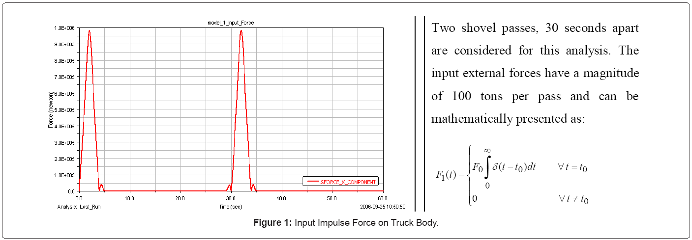
In the MSC.ADAMSenvironment, the applied forces are input into the model. These forces are the external excitations on the truck system under the HISLO conditions, and thus, they correspond to the load dumped by the shovel under gravity. These input forces acting on the truck body are impulsive and time dependent. They fall under the “Custom Forces” category in MSC.ADAMS. The magnitude of these forces is a user-written subroutine that defines a non-standard input into ADAMS, using the AKISPL data access subroutine. AKISPL uses the Akima cubic-curve fitting method of interpolation to create a spline function across a set of data points. The data points to be interpolated are defined by a SPLINE statement in the ADAMS/Solver dataset. The user-defined SPLINE in the dataset represents the impulse force that changes with respect to time. The ADAMS/Solver uses the cubic polynomial to interpolate between points. The AKISPL function is very fast, and always produces accurate results for the value of the approximated function. The impulse input force is illustrated in figure 1.
AKISPL returns estimates for the first derivative of the approximated function with evenly spaced data points. After assigning the input forces, MSC.ADAMS/View evaluates the reactive forces on the structure that corresponds to the spring-damper systems. It also evaluates the reactions in the joints connecting different components due to the dynamic motion of the structure under the input force. Once the 3D virtual model is built and validated, a static simulation is performed to configure the model under equilibrium conditions. It is then followed by a dynamic simulation, which reduces some of the initial, transient system responses. During the static equilibrium simulation process, the Adams/Solver iteratively adjusts the spatial geometry of all the parts to balance all the forces on the system. A static simulation is performed with initial conditions to check and correct any geometric inconsistencies in the model. The corrected model becomes an input for a nonlinear or linear simulation.
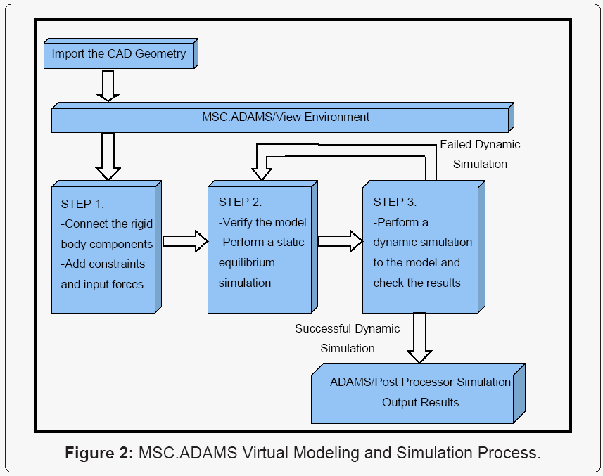
Once the static simulation is completed, a dynamic simulation is carried out. During this simulation process, Adams/View (i) sets the initial conditions for all the model objects, (ii) formulates appropriate equations of motion (EOM) based on the laws of Newtonian mechanics. The EOMs control objects motions given the set of forces and constraints acting on them, (iii) solves the EOMs for component displacements, velocities, acceleration, and the applied and constraint forces to within the specified accuracy tolerance, (iv) temporarily saves the results for later animations, plots, and numerical signal processing. The animations provide graphical illustration of the overall behavior of the model for pinpointing specific problems, such as improper connectivity or misapplied motions or forces. ADAMS/View can display this information in strip charts through measures. ADAMS/ Post Processor displays the results for more in-depth investigation and manipulation. Figure 2 illustrates the stages and procedures for developing and simulating the virtual prototype simulator of the HISLO problem.
After importing the CAD geometry into the MSC. ADAMSenvironment, the first step consists of connecting the elements together and adding the constraints to the model that mimics the physical constraints of the actual truck. Then, the static equilibrium simulation is performed to verify the stability of the model. The third step is to perform a dynamic simulation by defining the simulation end time and the step size. If the simulation is successful, the results are viewed in ADAMS/Postprocessor. If the simulation fails, the model is verified again for stability, constraints and proper joints selection.
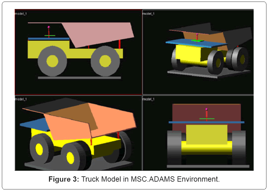
Figure 3 shows different views of the 3D virtual prototype model of the truck developed in ADAMS/View.CAT 793D dump truck parameters and dimensions are used in this analysis. It also shows the connections between the different parts via springs and dampers. The ground is showed as a plate with unit thickness. The operator is modeled as two elements, his neck and body are connected via springdamper system. The result is a 37-DOF virtual truck model that can be simulated under various conditions, which includes the HISLO.
Dimensions constraints and control environment
The overall 37-DOF virtual truck model experiences constraints from dimensions to control environment. The attachments serve as the physical bearings and bolts in the truck. These attachments, or joints in MSC.ADAMS, add constraints to the overall model by defining the geometric relationships (i.e., joints) and the relative motions of the system components. These joints allow motion in any of the six axes, three for translation and three for rotation. The joint motions and their impact on the different rigid components of the truck model determine the overall number of degrees of freedom of the truck. For instance, the truck bed is attached to the chassis and rotates around the y-axis while it is constrained in the three translational and the other two rotational axes. The dimensions of the different components are set in the CAD environment, while constructing the geometry of the truck. These dimensions are unchanged in MSC.ADAMS. However, the mass properties, such as densities and Poisson’s ratio, must be modified in order to maintain similar properties as the physical components in the truck. This is required to create a solid geometry that mimics the actual truck instead of a shell with no properties.
The control environment for the virtual model consists of maintaining static equilibrium by connecting all parts to each other with one part connected to a fixed reference. This fixed reference is essential for successful simulation and to avoid free falling parts due to the presence of gravity. Thus, the connections between the parts are achieved by adding spring and damping controls to the model. These controls introduce forces that resist the motion. The characteristics of these forces, created by MSC.ADAMS/View, are based on the stiffness and damping coefficients specified by the user. In this case, MSC.ADAMS/View automatically generates forces with magnitudes proportional to the distance and velocity between two points. The coefficients specified by the user represent the proportionality constants. Moreover, the joints return a reactive force on one of the two bodies connected by the joint object. Also, the impulsive force generated under the HISLO conditions is input as a SPLINE data element function that defines a curve defining the force magnitude with respect to time. This force has a single component in the vertical direction and is constrained in the other five directions (two translational and three rotational) as illustrated in figure 1.
Methods in MSC.ADAMSenvironment
The MSC.ADAMS/Vibration environment is a plug-in to MSC. ADAMS/Solver and MSC.ADAMS/View that allows the performance of the frequency-domain analysis of forced vibrations over different operating points in order to compute the system response. MSC. ADAMS/Vibration plug-in evaluates the frequency response functions for magnitude and phase characteristics and solves for the system modes over the frequency range of interest. It also tabulates the contribution of the model elements to the kinetic, potential, and dissipative energy distribution in the system modes.
The two types of analyses used in this paper are the normal mode analysis and the forced response analysis. The normal mode analysis computes the Eigenvalues and Eigenvectors of the model at a specified operating point set by the user. This analysis is effective in understanding the natural modes of vibration for the model and to determine the basic dynamic characteristics of the model. Although the results of the Eigenvalue analysis are independent of the external excitation, they are useful in predicting the effects of applying dynamic loads to the model. The normal mode analysis is relevant in the determination of the natural frequencies of the truck model. On the other hand, the truck vibration problem, under the HISLO conditions, consists of a forced vibration problem. Therefore, the forced response analysis is performed for the virtual prototype dynamic analysis. The forced response analysis is the response of the model to vibration input channels that describes the input excitation on the system. This forced response analysis consists of a collection of input and output channels, the operating point specification, the frequency range and number of steps in this range.
Forced response analysis in MSC.ADAMS: ADAMS/Vibration requires the definition of a collection of input and output channels, the operating point, the frequency range and the number of steps in this range in order to perform a forced-response vibration analysis. A vibration input channel defines the location, orientation, and the type of the applied forced function. The type of input channels that corresponds to the HISLO conditions specified in ADAMS/Vibration is the force-type input channel. The vibration output channels are defined using run-time expressions (MSC.ADAMS, 2007). These expressions can consist of kinematic or forced expression or some combination of the state variables defined by the user. The system of differential and algebraic equations is linearized about an operating point z0. An operating point is defined by an initial-conditions analysis or static or dynamic analysis [5].
The Eigenvalue problem is solved in ADAMS/Vibration using the well-known QR method [6] for computing Eeigenvalues and Eigenvectors. The integrator statement controls the numerical integration of the EOMs for a dynamic analysis. ADAMS/Solver (FORTRAN) uses an iterative, quasi-Newton-Raphson algorithm to solve the difference equations and obtain the values of the state variables. This algorithm ensures that the system states satisfy the EOMs. The Newton-Raphson iterations require the Jacobian matrix, which are the partial derivatives of the equations being solved with respect to the solution variables. The GSTIFF (Gear integrator) is the default integrator used by ADAMS/Solver (FORTRAN) for integrating the differential EOMs. The GSTIFF default integrator uses Newton- Raphson iterations to solve the nonlinear Differential-Algebraic Equations (DAE) of motion. It is a variable-order, variable-step and multi-step integrator with a maximum integration order of six. The Backward-Difference Formulae (BDF) coefficients are calculated by assuming that the step size of the model is mostly constant. Thus, when the step size changes in this integrator, a small error is introduced in the solution. The RKF 45 method is chosen as the integrator used by ADAMS/Solver because it is suitable for solving non-stiff vibration problems and gives accurate results for the acceleration fields.
Numerical method used in MSC.ADAMS: The RKF 45 method is used to integrate the differential equations governing the system. It is a single-step method, which is primarily designed to solve nonstiff and mildly stiff differential equations when derivative evaluations are not expensive or time consuming. Internally, RKF 45 uses the DDERKF code, which is a driver for a modification of the RKF 45 code by Shampine and Watts [7]. The RKF methods are an extension of the traditional Runge-Kutta (RK) methods. The local truncation error per step for the RKF method is computed by comparing the calculated result, yn+1 (at t=tn+1), with the result of an associated higher order RK formula. Therefore, in a fourth-fifth order method, the error in the fourth-orderRK method is estimated by subtracting it from the value obtained by a fifth-order RK method. In its formulation in ADAMS/ Solver, the derivative evaluation is time consuming; thus, RKF 45 is usually not very fast. The RKF 45 is about five times slower than the default GSTIFF for most models. However, RKF 45 is a good addition to the suite of integrators in ADAMS, because, unlike all the others, it is a single-step integrator. It can only handle ODEs and not Differential Algebraic Equations (DAE). Therefore, the DAE equation of the model needs to be transformed into ODE.
The RKF 45 uses coordinate partitioning to convert the DAE into ODE. This is achieved by using the coordinate partitioning, which is a method of eliminating constraint equations, such as the ones induced by joints, from the EOMs. This method reduces the entire system of DAEs to a condensed set of ODEs. It does so by selecting the degrees of freedom that will change the most during the simulation constraints. After each successful integration step, the coordinate-partitioning algorithm computes the dependent displacements, their time derivatives, and the accelerations and Lagrange multipliers (constraint reactions). During this process, ADAMS/Solver (FORTRAN) holds the independent coordinates constant and employs a Newton-Raphson iteration scheme to find the dependent coordinates. After computing the dependent velocities from the independent values, the ADAMS/ Solver uses the Newton-Raphson algorithm again to find the full set of accelerations and Lagrange multipliers.
The different stages for solving the complete vibration problem of the truck model under HISLO conditions are by using ADAMS/ View for dynamic simulation analysis; followed by a modal and forced response analyses using MSC.ADAMS/Vibration. Finally, MSC. ADAMS/Post Processor is used to post-process the results, such as debugging, validating, improving and presenting the results. Postprocessing involves animating forced vibrations and plotting frequency response functions, generating modal coordinates, and displaying other time and frequency data.
Limitations of the virtual model
The virtual model of the truck vibrations simulator has limitations in the input parameters, as well as, the simulation process as described in the sections below.
Input parameters limitations: The input parameters introduce limitations in the overall solution of the HISLO vibrations problem due to the data unavailability. There is no published data for the stiffness and damping coefficients for the CAT 793[8] truck series. These coefficients are approximated based on the available literature for heavy machinery and farming trucks [9], as well as, data from Caterpillar (2007). These parameters, once defined for a specific dump truck, such as the CAT 793 and the CAT 797 series, can be input into the generic simulator for formulating the model under HISLO conditions.
Simulationlimitations: The RKF 45 integrator is used to solve the multi-degrees of freedom vibration problem under the HISLO conditions. Thus, the simulation is five times slower than the default MSC.ADAMS/Solver. The computation time might be too costly for solving the 37-DOF truck model in industrial applications. Also, the RKF 45 can only handle ODEs, and not DAE. Therefore, the DAE corresponding to the model needs to be transformed to ODE. The RKF 45 is suitable for the vibration analysis but is only supported by the FORTRAN77 solver. Therefore, kinematic analysis on critical models cannot be performed. This type of analysis is supported by the C++ Solver because it uses a more advanced quadrature scheme to integrate the motion function. This is a potential source of difference in the results produced by the two solvers.
Confidence in the simulated results: The confidence level is the measure of how reliable are the simulation results compared to the real-world scenario. The results are expected to be at 95% confidence level. Due to the fact that the stiffness and damping coefficients are approximated based on the suspension cylinder stroke, the simulation results will be different than the experimental results. Comparing the simulation results with the experimental data [10] under the same operating conditions, the differences are in the range of 1% to 9% (Table 1).
| RMS Acceleration (m/s2) | Virtual Prototype Results | Kumar’s (1999) Results | Percent Difference (%) |
|---|---|---|---|
| Cervical Region | |||
| ax | 0.36 | 0.35 | 2.8 |
| ay | 0.53 | 0.52 | 1.9 |
| az | 0.87 | 0.84 | 3.4 |
| Lumbar Region | |||
| ax | 0.40 | 0.38 | 5.0 |
| ay | 0.42 | 0.41 | 2.4 |
| az | 1.12 | 1.09 | 2.7 |
| Operator Seat | |||
| ax | 1.49 | 1.47 | 1.3 |
| ay | 1.08 | 1.19 | 9.2 |
| az | 3.56 | 3.49 | 2.0 |
Table 1: RMS Accelerations Comparison between ADAMS and Experimental Results.
Conclusion
A detailed description of the techniques and methods has been provided for building the virtual model in the MSC. ADAMSenvironment. The process begins by exporting the CAD geometry of the truck into ADAMS. System constraints were added to the ADAMS model in order to replicate the physical behavior of the truck model under the HISLO conditions. The Akima cubic-curve fitting method of interpolation was used to create a spline function using a set of data points. This spline function generates a curve that models the high material impact into the truck body under gravity. Static equilibrium simulation was performed to verify the model’s consistency before carrying out the dynamic simulation. The dynamic simulation of the 37-DOF truck model, under the HISLO conditions, is carried out by using the RKF 45 algorithm and the FORTRAN solver.
This paper discusses the details of the development and simulation of a generic truck 3D virtual model. This generic model can be used to simulate the vibration of any truck provided that the masses, stiffness and damping coefficients are available. The simulation limitations consist of the slow computation of the solution using RKF 45 integrator that is only supported by FORTRAN solver, but is suitable for the vibration analysis of the truck model under HISLO conditions. Comparing results between the simulated 3D virtual prototype truck model and experiments conducted in the field, shows 1% to 9% difference in the root mean square (RMS) acceleration at key positions defined by the researcher. Hence, the 3D virtual model can be used as a simulator tool under various conditions to predict acceleration results where experiments become costly in terms of time and money.
References
- MSC.ADAMS (2007) MSC Software Corporation. MSC.ADAMS Santa Ana, CA, USA.
- ISO 2631-1 (1997) Mechanical Vibration and Shock-Evaluation of Human Exposure to Whole-Body Vibration-Part 1: General requirements. International Organization for Standardization, Switzerland.
- ISO 2631-4 (2001) Mechanical vibration and shock-Evaluation of human exposure to whole-body vibration-Part 4: Guidelines for the evaluation of the effects of vibration and rotational motion on passenger and crew comfort in fixed-guideway transport systems. International Organization for Standardization, Switzerland.
- ISO 2631-5 (2004) Mechanical vibration and shock-Evaluation of human exposure to whole-body vibration-Part 5: Method for evaluation of vibration containing multiple shocks. International Organization for Standardization, Switzerland.
- Sohoni VN, Whitesell J (1986) Automatic Linearization of Constrained Dynamical Systems. ASME 108: 300-304.
- Press WH, Teukolsky SA, Vetterling WT, Flannery BP (1992) Numerical Recipes in FORTRAN: The Art of Scientific Computing. (2nd Edn) Cambridge University Press, England, UK.
- Shampine LF, Watts HA (1979) Design of a User Oriented Package of ODE Solvers. Technical Report Sand, DEPAC Sandia National Laboratories, Albuquerque, New Mexico, USA.
- Caterpillar (2007) CAT Performance Handbook. Illinois, USA.
- Trangsrud C, Law E, Janajreh I (2004) Ride Dynamics and Pavement Loading of Tractor Semi-Trailers on Randomly Rough Roads. SAE Technical Paper 23-46.
- Kumar S (1999) A Study of: Effect of Vibration and Impact on Drivers of Heavy Haulers in Winter Conditions at Syncrude. Department of Physical Therapy, Faculty of Rehabilitation Medicine, University of Alberta, Edmonton, Alberta, Canada.
Relevant Topics
- Additive Manufacturing
- Coal Mining
- Colloid Chemistry
- Composite Materials Fabrication
- Compressive Strength
- Extractive Metallurgy
- Fracture Toughness
- Geological Materials
- Hydrometallurgy
- Industrial Engineering
- Materials Chemistry
- Materials Processing and Manufacturing
- Metal Casting Technology
- Metallic Materials
- Metallurgical Engineering
- Metallurgy
- Mineral Processing
- Nanomaterial
- Resource Extraction
- Rock Mechanics
- Surface Mining
Recommended Journals
Article Tools
Article Usage
- Total views: 15439
- [From(publication date):
specialissue-2013 - Dec 04, 2024] - Breakdown by view type
- HTML page views : 10981
- PDF downloads : 4458


