Research Article Open Access
Tracking Knee Joint Functional Axes through Tikhonov Filtering and Plucker Coordinates
| Wangdo Kim1, Yoon Hyuk Kim2, António P Veloso1 and Sean S Kohles3* | |
| 1Univ Tecn Lisboa, Fac Motricidade Humana, CIPER, LBMF. Estrada da Costa, P-1499-002 Lisbon, Portugal | |
| 2Department of Mechanical Engineering, Kyung Hee University, Yongin, 446-701, Korea | |
| 3Regenerative Bioengineering Laboratory, Departments of Mechanical and Materials Engineering and Biology, Portland State University, Portland, OR, USA | |
| Corresponding Author : | Sean S Kohles, PhD Adjunct Professor Departments of Mechanical and Materials Engineering and Biology Portland State University, P.O. Box 751 Portland, OR, USA, 97207-0751 Tel: 503-516-7528 E-mail: kohles@pdx.edu |
| Received December 26, 2012; Accepted February 27, 2013; Published March 01, 2013 | |
| Citation: Kim W, Kim YH, Veloso AP, Kohles SS (2013) Tracking Knee Joint Functional Axes through Tikhonov Filtering and Pl�?±cker Coordinates. J Nov Physiother S4:001. doi: 10.4172/2165-7025.S4-001 | |
| Copyright: © 2013 Kim W, et al. This is an open-access article distributed under the terms of the Creative Commons Attribution License, which permits unrestricted use, distribution, and reproduction in any medium, provided the original author and source are credited. | |
Visit for more related articles at Journal of Novel Physiotherapies
Abstract
Researchers have reported several compensation methods to estimate bone and joint position from a cluster of skin-mounted markers as influenced by Soft Tissue Artifacts (STA). Tikhonov Regularization Filtering (TRF) as a means to estimate Instantaneous Screw Axes (ISA) was introduced here as a means to reduce the displacement of a rigid body to its simplest geometric form. Recent studies have suggested that the ISA of the knee, i.e., Knee Functional Axes (KFA), might be closely connected to the estimation of constraint forces such as those due to medial and lateral connective tissues. The estimations of ISAs were known to be highly sensitive to noisy data, which may be mathematically ill-posed, requiring smoothing such as that conducted by regularization. The main contribution in this work was to establish the reciprocal connection between the KFA and Ground Reaction Forces (GRF) as a means to estimate joint constraint forces. Presented results compare the computational performance with published kinetic and kinematic joint data generated from an instrumented total knee replacement. Implications of these preliminary findings with respect to dynamic alignment as a functional anatomic metric are discussed.
| Keywords |
| Dynamic alignment; Instantaneous screw axes; Knee biomechanics, L-curve method; Osteoarthritis; Regularization; Soft tissue artifact |
| Introduction |
| The strategies for minimizing modelling errors such as those produced by Soft Tissue Artifacts (STAs) have received much attention from both researchers and practitioners [1,2]. Techniques designed to minimize the contribution of and compensation for STAs can be divided into those which model the skin surface and those which include joint motion constraints. A “solidification” procedure was proposed recently based on the assumption that marker trajectories are consistent with the rigid body motion [3]. A different approach corresponds to principal axes of inertia in which each segment marker is assigned a mass that can act as a Probability Density Function (PDF) or weighting factor [4]. The Centre of Mass (COM) and the inertial tensor of the marker-clusters are calculated at each time frame. This technique is based on the analogy that the inertial tensor about the COM of a Three-Dimensional (3D) rigid body is related to the covariance matrix of the trivariate random vectors, whose PDF is proportional to the point-wise density of the rigid body itself. The global optimization treats each body segment in holistic terms, i.e., a structure that is undergoing transformation as a whole, rather than in terms of separate segments each with imposition constraints at the joint [5]. This process has been defined by minimizing the weighted sums-of-squares distance between simulation and model-determined marker positions. |
| The described compensation techniques all have common features. The transformation parameters (both rotation and translation) can be computed from linear interpolation as is done for affine mapping. Subsequently the Least-Squared Estimates (LSE) can be adopted by means of extracting transformation parameters between two point patterns via Singular Value Decomposition (SVD). However, the LSE is not a sufficient estimate as the ultimate solution minimizes the error and concludes with the model exactly matching the data. Since the marker data are assumed to have position errors, the analysis objectives are not satisfied during STA compensation. Estimating Instantaneous Screw Axes (ISA) from noisy data was originally defined as an example of the ‘inverse problem’ facing an ill-posed biomechanical scenario [6], where the regularization theory and projective geometry were proposed for solving these types of problems. The duality between the pure rotation and translation can become diminished in Euclidean space where parallelism and infinitely distant quantities create difficulties. The duality is, however, perfect in projective geometry, where infinite quantities are on an equal basis with finite ones. Plűcker coordinates are perhaps the most versatile realization of screw quantities and capture that duality. Here, the regularization method provides an enhanced analytical tool for improved STA compensation [7]. |
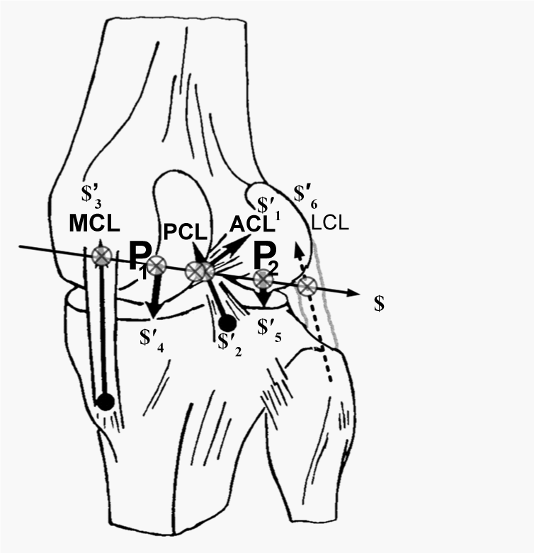
| In the following study, we estimated spatial-temporal knee joint motion by incorporating a novel approach for STA compensation through the application of the L-curve Tikhonov Regularization Filtering (TRF) algorithm. The importance of accurately locating the Knee Functional Axis (KFA) through enhanced analytical approaches was one of the key lessons developed during the 2010 ASME Grand Challenge Competition to predict in vivo Knee Loads [8]. These changes in position and orientation of the KFA should be considered in the analyses of muscle function during human movements (which require moment arms to be defined relative to a functional axis of rotation). In particular, the reciprocal connection theory indicates that the ligaments and cartilage contact contribute to the mechanical constraints within knee joints (Figure 1), which results in a KFA that was also reciprocally connected to the Ground Reaction Forces (GRF) from our view [9]. |
| Therefore, our investigation tests the hypothesis that the technical approach described herein can correctly locate the KFA in the global reference frame, which can in turn be associated with a qualitative/ quantitative estimation of joint constraint forces. The first aim of the present study was to compensate for the STA by the TRF approach to generate the ISA and correctly locate the KFA. The second aim of our study was to apply the KFA tracking that we obtained, combined with the corresponding GRF tracking as a reciprocal connection, toward the estimation of knee constraint forces for clinical applications [9,10]. We then verify this approach by comparing results obtained in terms of KFA with in vivo knee loads measured directly from an instrumented total knee implant. |
| Materials and Methods |
| Analytical model |
| Inverse mechanics equations and the L-curve method were previously applied to estimate the optimal values of the smoothing parameters during multi scale cell-tissue level [11] and joint level [9] biomechanical analyses. A similar technique was applied here to compensate for the STA during the study of joint biomechanics. Briefly, we applied a third-order model that estimated the first and second time-derivatives of the data. The formulation of the discrete inverse problem can be stated in terms of the state variable vector z j , which represents the position x, velocity v and acceleration a of marker points at time j. The kinematic parameters are: |
| which are driven by the forcing function g(t), which is not associated with gravitational acceleration. The discrete model then becomes: |
 (2) (2) |
| Where h represents a sampling time step. The error term is a combination of matching the data dj and the regularization of gj. The LSE error term is now expressed as: |
 (3) (3) |
| This function identifies the minimum error value of E starting at any stage j = n with x n = c and simulating the system to the end condition( j = N ) with the optimal ′g j s then being defined. The important items to emphasize are that c is considered to be arbitrary and that n can represent any value between 1 and N. |
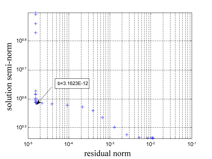
| What is now required of the solution is to best match the data (the first term of Equation 3), while maintaining some degree of smoothness (the second term of Equation 3). By adding a term to the LSE error function in Equation 3, one can control the amount of smoothness that occurs in the solution by varying the parameter b. The analytical smoothing problem is then to find the forcing term gj and the initial condition c that minimizes the error function EN while also determining the optimal values of the smoothing parameter b. The addition of the term bg2 j is crucial to obtaining smooth and reasonable results. This approach is known as regularization for numerical smoothing and accuracy control, and is sometimes referred to as the Tikhonov method. The method for estimating the optimal value of b is called generalized cross validation or the Tikhonov L-curve approach [12]. Other methods used Morozov’s discrepancy principle for Tikhonov regularization for solving ill-posed problems [13]. The L-curve displays information about the regularized solution by plotting the iterative solution of Equation 3 versus the residual vectors (the deviation between observed and predicted values) typically on semi-logarithmic axes. In the simplified application here, a scalar of the regularization parameter b was chosen by identifying the characteristic reflection point on the generated plot. |
| In essence, it is desired to find the input driving force gj that causes the model xj to match the data dj as closely as possible. Thus, the analysis minimizes the function EN over the sequence of forcing vectors gj. The inverse (filtering) problem is then to find the unknown force gj that minimizes the errors expressed in Equation 3 while using the model of Equation 2. This approach can also be thought of as an optimal control problem with gj as the controlling forces. The mathematical problem can be solved using dynamic programming and Bellman’s Principle of Optimality [12] and produces the equation: |
| which is a recurrence formula described in previous biomechanical applications by others [14]. |
| Line coordinates (or Plücker Coordinates) were extended here to describe screw motion (rotation with translation) and applied to locate the KFA [15]. The coordinate system of the screw axis $ is then written as: |
| The variables L,M,N represent the orientation of the axis of $; and the variables P,Q,R define the moment vectors of $. When normalized by L2 +M2 + N2 =1 such that L = L,M = M and N = N , the two sets of coordinates are related by a scalar multiplier ρ : |
| A unit screw is then defined to which no mechanical significance is attached until a twist (wrench) of scalar amplitude (intensity) ρ is associated with it. As expressed in equation 6, a screw when considered as a geometric element, is then defined by the relative and not the absolute value of its coordinates, thusly named the homogeneous coordinates. |
| Knee biomechanics application |
| Knee biomechanics application The method that determines the ISA in terms of screw coordinates from the rigid body transformation was applied here to estimate the ISA from filtered data [16]. The screw axis attached to the shank limb segment will trace out a ruled surface, a set of screws $1for the shank, similarly,$2 for the thigh limb segment. Uniform motion transmission (without disengagements) between two generally disposed axes is possible only if: |
| Where dv1 $1 is the displacement of the shank, dv2 $2 is the displacement of the thigh, and dvKFA $KFAis the relative displacement of the thigh with respect to the shank, which is also defined as the KFA. The Arhnold-Kennedy theorem applied to three axes may be manifested as the two ISAs $1 and $2 , resulting in a third ISA $KFA on the cylindroid defined by a linear combination of the two axes [17]. Solving equation 7 is equivalent to locating the KFA. The reciprocal connection theory was applied to predict the reaction of constraints evoked when the GRFs were accessible during the stance phase [9]. |
| The principle of virtual work for static equilibrium, which states that the virtual work of the GRF applied on the knee in equilibrium with workless constraint is equal to zero, enables us to predict the intensities of constraint forces by connection of the latter to the location of the KFA. The GRF can then be decomposed into components of their three screws, the medial, lateral, and muscle forces, collectively acting on the KFA. It is always possible to determine wrenches on the four screws which are in equilibrium, and the ratios of their intensities alone are then determined [18]. |
| In order to attain the continuous estimation of forces in the course of the gait cycle, the excursion in KFA tracking needs to be generated and combined with the corresponding GRF. A comprehensive data set was accessed to determine the KFA during gait. This data set included motion capture, ground reaction, electromyography, tibial contact force, and strength data [19]. This experimental gait data were collected from an adult male subject (subject code JW) implanted with an instrumented total knee replacement (mass 68 kg, height 1.66 m, right knee) and analyzed using the described TRF approach at 50 ms time increments. Here, the ISA were generated using the previously described Plűcker Coordinate-technique [16]. The gait trial involved a medial-lateral trunk sway gait pattern similar to that previously reported [20]. Our study then used the following framework to predict reaction of constraints (Figure 4). The inputs were a reciprocally connected knee model, experimental kinematics (i.e., x-y-z trajectories of marker data at patella, shank and thigh), and ground reaction forces that were all obtained from the instrumented right knee of the subject. The “knee radiograph” contained a view of the knee region in the frontal plane and provided geometrical information about constraints. The algorithm for calculating reciprocal screws using the nullspace operation was originally developed by Konkar and Cutkosky [21] and later presented in detail using MATLAB functions (Mathworks, Inc., Natick, MA) by Adams and Whitney [22]. The algorithm has been used to describe the reciprocal connections of the KFA to the knee constraints [9]. A validation of this approach was conducted by directly comparing measured and predicted joint forces through time. |
| Results |
| Upon processing marker coordinates from the shank, the TRF plot indicated a distinct inflective corner, which was associated with the optimized value of the regularization parameter (Figure 2). Thus, the flexion point on the semi-logarithmic plot of the iterative solution versus the residuals was chosen as b=3.1623×10⁻¹². It was found that the ordinary process of estimation of b could not be applied to the optimal generation of knee instantaneous axes. The demarcation between our application and an ordinary filtering technique is that a filtering process takes place in real time, while most of our applications are based on the assumption that we have the entire set of measurements at our disposal instead of obtaining them one at a time and having to make instantaneous decisions. |
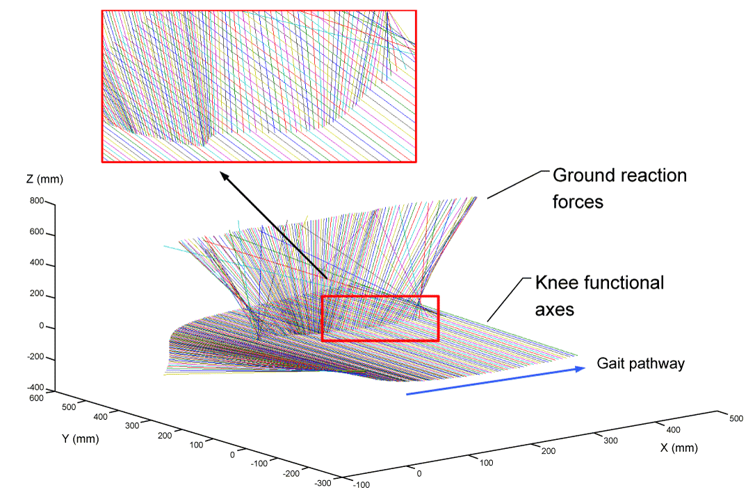
| The ISAs that were produced when the Tikhonov parameter was assigned asb=0.001 were plotted from a laboratory coordinate frame analysis in terms of the KFA as the gait cycle progressed (Figure 3). The KFA was determined by the linear combination of two ISA’s of the shank and thigh in equation 7. Moreover, by virtue of positioning the KFA of the knee in the global frame, those KFAs could be somewhat connected with the Ground Reaction Force (GRF) resident on the screws during gait trials. An impulsive force of constraint was evoked to define the intersection of the reciprocal connection with the correspondence between the GRF (zoomed image in Figure 3), where the KFA adds the geometrical factors to facilitate the interaction between the two screw surfaces. As the impulsive reaction forces and instantaneous screw exists, a one-to-one correspondence can be defined. To express this differently, the mechanical complex of instantaneous and that of impulsive screws are projective. |
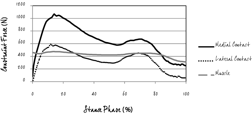
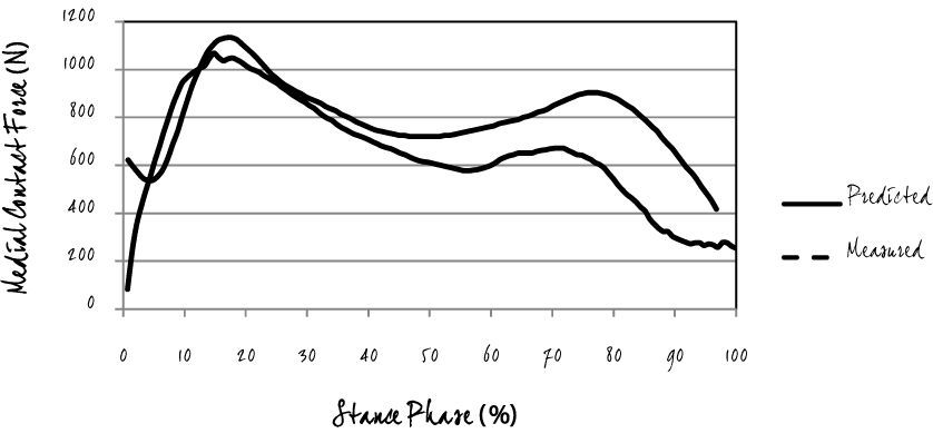
| In the biomechanical model presented in this paper, the contribution of the limb/body weights and accelerations were not included so that the smaller joint/tissue forces could be estimated. The forces in the medial and later compartments as well as a single muscle force are presented as a first approximation by applying the principle of virtual work for static equilibrium condition (Figure 4). It states that the virtual work of externally applied forces composed of muscles and GRF at the KFA in equilibrium with workless constraints is equal to zero. As noted, this resulted from decomposing the measured ground reaction forces to the corresponding constrains and muscle forces. The Root Mean Square (RMS) error for the medial contact force during the contact of the foot with the ground was determined to be 184.7 N (Figure 5). |
| Discussion |
| The purpose of this study was to obtain the desired excursion of the KFA by connecting the GRF to the joint constraint reaction forces in terms of a “reciprocal connection” paradigm. We satisfied our objectives and rejected the null hypothesis by demonstrating that KFA tracking, in terms of two screw-axis surfaces during the stance phase, is a purely geometric representation of the GRF-KFA interaction [23] and can reasonably represent joint mechanics. |
| While there were similarities between the prediction of this model and the validation measurements, there were also some profound differences. Similarities include the double peaked nature of the medial contact force curves. The knee joint loading pattern during the stance phase indicates two major peak force levels, the first peak occurring in early stance and the second peak occurring in late stance (Figure 4). This pattern was consistent with previous studies [24]. Here the medial compartment bears a greater proportion of the net load than the lateral compartment (Figure 4). Differences in the comparison include the fact that our model did not include inertias and the analysis was only performed at beginning of the joint motion routine due to impulses from static equilibrium [25] (Figure 5). |
| As a limitation, the parameter b, when optimized as a filter for the marker coordinates, could not accurately function as a smoothing parameter for the KFAs. For smoothing a ruled surface defined by the KFA trace, we arrived at a ‘b’ of 0.001 as a correct parameter via a trial-and-error approach. Different regularization parameters may result in distinctive control forces defining in equation 3. However, b will be affected by changes in both the shank and/or the thigh motion during gait. Several studies support the premise, as an important result of this study, that locating KFA is not directly related to the filtering of marker data alone, but rather to the gait environment. There are other methods such as representing joint displacement using a sequence of rotations about successive axes [26]. However, in that case, the difficulty for clinical applications is to correctly locate these axes such that they coincide with the anatomically functional axes of the considered joints. Our current view manifests that ligament and cartilage contact forces contribute to the mechanical constraints within knee joints, which result in KFAs and are reciprocally connected to GRFs. We consider the application of TRF with Plűcker coordinates as a powerful filtering strategy which combines the two well-established approaches. These include: (a) screw quantities in the field of ill-posed mathematical problems; and (b) the regularization technique, a general formulation of the inverse problem. |
| The presented approach could be extended as a measure of dynamic alignment, an indicator of risk associated with knee osteoarthritis progression. One can realign the GRF with the KFA by identifying an offset component reducing the load on the medial/ lateral compartment, thus redistributing the reaction (braking) torque about the KFA induced by the surrounding muscles. The reaction forces (and torques) of the GRF would then be shifted to the muscle reactions instead, guiding a therapeutic strategy. |
| In conclusion, the methods presented here enable us to obtain the desired KFA tracking that can be used to connect the instantaneous screw of the knee motion to the impulsive reaction force as a “dynamic alignment” technique. We demonstrated that KFA tracking is a purely geometrical factor describing the interaction between gait kinematics and ground reaction kinetics. Therefore, the shape of KFA tracking may be regarded as the “genome” of gait pattern recognition under all load-bearing physiological conditions. |
| Acknowledgements |
| This analytical work supports the ongoing research effort entitled “Orthopaedic Alignment & Screw Imaging Systems (OASIS)” as funded by the FCT (PTDC/DES/119559/2010). Experimental data were provided for validation through the Grand Challenge Competition to Predict In Vivo Knee Loads, a part of the Symbiosis Project funded by the National Institutes of Health (NIH) through the NIH Roadmap for Medical Research (Grant U54 GM072970). Author WK thanks his father, Doohoon Kim, for the introduction to screw theory. Author SSK also acknowledges support from the NIH (Grant P20 MD003350). |
References
- Leardini A, Chiari L, Della Croce U, Cappozzo A (2005) Human movement analysis using stereophotogrammetry. Part 3. Soft tissue artifact assessment and compensation. Gait Posture 21: 212-225.
- Pierce JE, Li G (2005) Muscle forces predicted using optimization methods are coordinate system dependent. J Biomech 38: 695-702.
- Cheze L, Fregly BJ, Dimnet J (1995) A solidification procedure to facilitate kinematic analyses based on video system data. J Biomech 28: 879-884.
- Andriacchi TP, Alexander EJ, Toney MK, Dyrby C, Sum J (1998) A point cluster method for in vivo motion analysis: applied to a study of knee kinematics. J Biomech Eng 120: 743-749.
- Lu TW, O'Connor JJ (1999) Bone position estimation from skin marker co-ordinates using global optimisation with joint constraints. J Biomech 32: 129-134.
- Woltring HJ, Huiskes R, De Lange A, Veldpaus FE (1985) Finite centroid and helical axis estimation from noisy landmark measurements in the study of human joint kinematics. J Biomech 18: 379-389.
- Tikhonov AN (1977) Solution of Ill-posed Problem. New York: John Wiley.
- Kim W, Veloso A, Tan J, Andrade C (2010) A Reciprocal Connection at Knee Joint. Paper presented at the ASME 2010 Summer Bioengineering Conference, Naples, FL, June 16-19.
- Kim W, Kohles SS (2012) A reciprocal connection factor for assessing knee-joint function. Computer Methods Biomech Biomed Engin 15: 911-917.
- Kim W, Veloso AP, Vleck VE, Andrade C, Kohles SS (2013) The Stationary Configuration of the Knee. Journal of the American Podiatric Medical Association 103: in press.
- Kim HJ, Fernandez JW, Akbarshahi M, Walter JP, Fregly BJ, et al. (2009) Evaluation of predicted knee-joint muscle forces during gait using an instrumented knee implant. J Orthop Res 27: 1326-1331.
- Trujullo DM, Busby HR (1997) Practical Inverse Anlaysis in Engineering. Boca Raton: CRC Press.
- Anzengruber SW, Ramlau R (2010) Morozov's discrepancy principle for Tikhonov-type functionals with nonlinear operators. Inverse Problems 26: 025001.
- Kim W, Tretheway DC, Kohles SS (2009) An inverse method for predicting tissue-level mechanics from cellular mechanical input. J Biomech 42: 395-399.
- Hunt KH (1990) Kinematic geometry of mechanism. Oxford: Clarendon Press.
- Kiat, Kim W (2006) Estimation of the axis of a screw motion from noisy data--a new method based on Plucker lines. Journal of Biomechanics 39: 2857-2862.
- Dooner DB (2002) On the Three Laws of Gearing. Journal of Mechanical Design 124: 733-744.
- Ball R (1998) A treatise on the theory of screws: Cambridge University Press.
- Fregly BJ, Besier TF, Lloyd DG, Delp SL, Banks SA, et al. (2012) Grand challenge competition to predict in vivo knee loads. J Orthop Res 30: 503-513.
- M�?¼ndermann A, Asay JL, M�?¼ndermann L, Andriacchi TP (2008) Implications of increased medio-lateral trunk sway for ambulatory mechanics. J Biomech 41: 165-170.
- Konkar R, Cutkosky M (1995) Incremental Kinematic Analysis of Mechanisms. Journal of Mechanical Design 117: 589-596.
- Adams JD, Whitney DE (2001) Application of Screw Theory to Constraint Analysis of Mechanical Assemblies Joined by Features. Journal of Mechanical Design 123: 26-32.
- Fuller EA (1999) Center of pressure and its theoretical relationship to foot pathology. J Am Podiatr Med Assoc 89: 278-291.
- Sasaki K, Neptune RR (2010) Individual muscle contributions to the axial knee joint contact force during normal walking. J Biomech 43: 2780-2784.
- Vaughan CL (2003) Theories of bipedal walking: an odyssey. J Biomech 36: 513-523.
- Ying N, Kim W (2005) Determining dual Euler angles of the ankle complex in vivo using "flock of birds" electromagnetic tracking device. J Biomech Eng 127: 98-107.
Figures at a glance
 |
 |
 |
 |
 |
| Figure 1 | Figure 2 | Figure 3 | Figure 4 | Figure 5 |
Relevant Topics
- Electrical stimulation
- High Intensity Exercise
- Muscle Movements
- Musculoskeletal Physical Therapy
- Musculoskeletal Physiotherapy
- Neurophysiotherapy
- Neuroplasticity
- Neuropsychiatric drugs
- Physical Activity
- Physical Fitness
- Physical Medicine
- Physical Therapy
- Precision Rehabilitation
- Scapular Mobilization
- Sleep Disorders
- Sports and Physical Activity
- Sports Physical Therapy
Recommended Journals
Article Tools
Article Usage
- Total views: 13002
- [From(publication date):
specialissue-2014 - Dec 21, 2024] - Breakdown by view type
- HTML page views : 8632
- PDF downloads : 4370
