Research Article Open Access
Traces of Long-Memory in Pre-Seismic MHz Electromagnetic Time Series-Part 1: Investigation Through the R/S Analysis and Time-Evolving Spectral Fractals
Dimitrios Nikolopoulos1, Demetrios Cantzos2, Ermioni Petraki1, Panayiotis H. Yannakopoulos1 and Constantinos Nomicos3*
1Piraeus University of Applied Sciences (TEI of Piraeus), Electronic Computer Systems Engineering, Petrou Ralli and Thivon - 250, GR-12244 Aigaleo, Greece
2Piraeus University of Applied Sciences (TEI of Piraeus), Department of Automation Engineering, Petrou Ralli and Thivon - 250, GR-12244 Aigaleo, Greece
3TEI of Athens, Department of Electronic Engineering, Agiou Spyridonos, GR-12243, Aigaleo, Athens, Greece
- *Corresponding Author:
- Dimitrios Nikolopoulos
Piraeus University of Applied Sciences (TEI of Piraeus)
Department of Electronic Computer Systems Engineering
Petrou Ralli and Thivon - 250, GR-12244 Aigaleo, Greece
Tel no: 0030-210-5381560
Fax: 0030-210-5381436
E-mail: dniko@teipir.gr
Received date: June 26, 2016; Accepted date: July 15, 2016; Published date: July 18, 2016
Citation: Nikolopoulos D, Cantzos D, Petraki E, Yannakopoulos PH, Nomicos C (2016) Traces of Long-Memory in Pre-Seismic MHz Electromagnetic Time Series-Part 1: Investigation Through the R/S Analysis and Time-Evolving Spectral Fractals. J Earth Sci Clim Change 7:359. doi: 10.4172/2157-7617.1000359
Copyright: © 2016 Nikolopoulos D, et al. This is an open-access article distributed under the terms of the Creative Commons Attribution License, which permits unrestricted use, distribution, and reproduction in any medium, provided the original author and source are credited.
Visit for more related articles at Journal of Earth Science & Climatic Change
Abstract
This paper reports characteristic pre seismic electromagnetic disturbances in the MHz range detected prior to seven significant earthquakes of M L ≥ 5.0 which occurred in Greece between 2009 and 2015. The whole data set was investigated through Rescaled Range (R/S) analysis and wavelet based spectral fractal analysis. The long-memory trends hidden in the analysed signals were investigated via the Hurst exponent (H). The R/S method indicated that in the majority of the segments of the investigated signals, the H - exponents were in the range 0.7-0.9. Several exponents were above 0.9. This is associated with persistency. In several segments, the Hurst exponent exhibited small variance. Noteworthy fluctuations were also found. In many cases the H - time fluctuations were independent of the time evolution of the associated electromagnetic signals. The spectral fractal method, being more suited for this purpose, highlighted the characteristic signals’ epochs, governed by long-lasting fractal organisation. The calculated Hurst exponents in the characteristic long-lasting fractal epochs were associated with medium anti-persistent behaviour or with continuous switching between anti-persistency and persistency. The H - exponents of the random fractal organised segments were mainly persistent. From the data presented in this paper, it is deduced that the R/S method provides additional information on the estimation of the Hurst exponent when combined with the spectral fractal method. Both techniques should be employed in sequential steps to enhance the precursory value of the results.
Keywords
R/S analysis; Spectral fractal analysis; MHz (Mega Hertz); Earthquakes
Introduction
Earthquakes are natural phenomena which are sometimes so devastating that can be compared to tsunamis and volcanic eruptions in regards to their negative impacts on social safety and the economy. What makes strong earthquakes more dangerous and disastrous, is not that they are inevitable when certain geophysical conditions are met, but that they are still extremely hard to predict [1]. Because of this, it is still a significant goal of the earthquake scientific community to discover credible seismic precursors. However, despite the tremendous cumulative efforts in both the laboratory and the geophysical scales, the problem of earthquake prediction still remains elusive. Nevertheless, certain precursors have been recorded before specific earthquakes that provide scientific evidence of patterns that can be utilised as alarms of anticipating seismic events [1-7]. In anticipation of an earthquake rupture, certain preliminary activity can be expected if the observation is made in the near vicinity of a causative fracture [8]. The pre-seismic earthquake sequence consists of successive, magnitude-increasing events that become denser in time and space in an orderly fashion up until the main earthquake occurrence. Five expectation phases are usually considered. The first is the foundation stage which refers to the generation of maps with all the potential regional sites, where the highest in magnitude and repetition rate seismic events are recorded. Four ensuing stages, not strictly distinct, realise the earthquake prediction; they differ in the time interval that triggers an alarm and are categorized as precursors of long-term (up to 10 years), intermediate-term (1 year), short-term (approximately 36 days to 3.6 days) and immediate term (approximately 9 hours or less) types. Such separation into stages is dictated by the character of the process that leads to a strong earthquake and by the needs of earthquake preparedness; the latter comprises a range of safety measures for each stage of prediction [9]. In another approach, according to [10] the prediction of earthquakes can be classified into three different groups, the long-term (time-scale of 10 to 100 years), the intermediate-term (time-scale of 1 to 10 years) and the short-term. Note that even in short-term prediction there is no one-toone correspondence between abnormalities in the recordings and the seismic activity [1,2,11]. Albeit considerably more troublesome than the long-term and the intermediate-term predictions, the short-term prediction of earthquakes on a time-scale of hours, days or weeks, is considered to be of utmost importance for residents of high seismicity territories.
The short-term pre-seismic precursors that emerge due to the changes in the electromagnetic (EM) field of the geo-atmospheric environment are promising tools for earthquake prediction. Different studies have demonstrated that pre-seismic EM disturbances are detectable in a wide frequency band extending from few Hz to several MHz. Regardless of the investigative endeavours; the preparation and evolution of earthquakes is not fully deciphered yet. A critical reason is that there is limited knowledge of the breaking mechanisms of the crust [11-13] as every seismic event is case specific and happens in an extensive scale. Considering that the crack of heterogeneous materials is not adequately depicted yet [12], it can be comprehended why the determination of the beginning of an earthquake sequence is still constrained [11-27,29-34]. As per [12] one ought to expect that the preliminary procedures of earthquakes have different aspects, which might be witnessed before the final rupture at land, geochemical, hydrological and natural scales [12]. While each of these phenomena has been observed prior to certain earthquakes, such observations have been random in nature [1,35]. Finally, it is essential to note that ultralow (ULF), low (LF), high (HF) and very high frequency (VHF) EM irregularities have been observed over periods extending from a couple of days to a couple of hours preceding destructive land earthquakes or strong and shallow undersea earthquakes [11-23,25-27,29-34]. This paper concentrates on significant, short-term disturbances of natural EM radiation in the MHz frequency range. These were almost continuously recorded by a group of telemetry EM radiation stations that operates in Greece [36]. Special consideration was given to parts recorded up to one month before noteworthy earthquakes occurred in Greece. The principal aspect under investigation is to determine if fractal and long-memory trends exist in fragmented parts of these EM irregularities and assessing these, henceforth, as credible forerunners of general fracture. As analysed later, these trends are investigated through the time evolution of the Hurst exponent of pre-seismic EM time-series. The Hurst exponent is calculated through the Rescaled Range (R/S) method [37,38] and through fractal analysis based on the wavelet power spectral density (PSD).
Critical information derived from data spanning years 2009-2015 is presented in this paper. The investigation includes some significant undersea earthquakes and moreover, some noteworthy seismic events at shallow depths. The precursory value of all the results is discussed.
Materials and Methods
Experimental methods
Earthquakes analysed: Greece is a country prone to earthquakes because it is bounded by the regions of convergence of the Eurasian and African plates and the western termination zone of the North Anatolian Fault (Figure 1). The country is dominated by extensional seismicity structures and numerous active faults (http:// gredass.unife. it/) of complex active stress field (http://www.cprm.gov.br/33IGC/ 1344073.html). The seismicity structures evoked several earthquakes of ML ≥ 5.0 during the last century.

Figure 1: Plates bounding Greece.
Table 1 presents collectively the data of the earthquakes analysed. The epicentres, the coordinates and the dates of these earthquakes are given. The corresponding events are shown in Figure 2. As can be observed from Figures 1 and 2, the earthquakes 2, 3 and 4 occurred within the Hellenic Trench and especially earthquake 3 occurred within the outer non-volcanic arc. Earthquake 1 occurred in the area between the Aegean and the Anatolian Plates and earthquake 7 in the area between the Aegean and the Eurasian Plates. The remaining earthquakes, viz., the earthquakes 5 and 6 occurred in the Aegean Plate which is the main plate that covers Greece. Under this view, the earthquakes of this study were distributed along Greece. In addition, as can be observed both from
| Event | Date (Y/M/D) | Location | Latitude (0N) | Longitude (0E) | Depth (km) | Magnitude (ML) |
|---|---|---|---|---|---|---|
| 1 | 2014-05-24 | 22.9 km SSW of Samothraki | 40.29 | 25.4 | 28 | 6.3 |
| 2 | 2009-07-01 | 111.2 km SSE of Iraklion | 34.35 | 25.4 | 30 | 508 |
| 3 | 2014-08-29 | 69.4 km W of Milos | 36.67 | 23.67 | 97 | 5.7 |
| 4 | 2015- 04-17 | 67.2 km SSW of Karpathos | 35.16 | 26.74 | 40 | 5.4 |
| 5 | 2009-05-24 | 36.0 km NNW of Kilkis | 41.3 | 22.74 | 23 | 5.1 |
| 6 | 2014-08-22 | 50.6 km S of Poliyiros | 39.92 | 23.46 | 29 | 5 |
| 7 | 2009-01-08 | 139.9 km NNW of Florina | 41.94 | 20.74 | 2 | 5 |
Table 1: List of earthquake events which were analyzed in this study. (The numbering is in descending order of local magnitudes).

Figure 2: Locations of the analysed earthquakes. The colour index is identical to the one employed by the National Observatory of Athens, Institute of Geodynamics.
Table 1 and Figure 2, the seismic events which were used in this study had depths from 2 Km to 97 km, namely they were shallow, as well as, mid and deep undersea earthquakes. It is important to note also that, the selected seismic events had local magnitudes ML ≥ 5.0 (Table 1). The criterion for choosing these earthquakes was that the risk of such earthquakes can be excessive for human life. The numbering of the earthquakes in this table will be used hereafter as a reference for the analysed earthquakes.
Instrumentation: As mentioned, the earthquakes were analysed through MHz EM time-series. The MHz EM signals were continuously monitored by a telemetric network, which consists of 12 stations [36]. These stations were recently updated and are located in the following seismic regions: (1) Ithomi (O), Peloponnese, (2) Valsamata (F), Kefalonia Island, (3) Ioannina (J), (4) Kozani (K), (5) Komotini (T), (6) Kalloni (M), Lesvos Island, (7) Rhodes (A), Rhodes Island, (8) Neapolis (E), Crete Island,(9) Vamos (V), Crete Island, (10) Corfu (P), Corfu Island, (11) Ileia (I), Peloponnese and (12) Atalanti (H). Stations 1, 2, 9, 10 and 11 are located along the Hellenic Trench. Stations 5, 6, 7 are located in the vicinity of the Anatolian Plate and stations 3, 4, 8 are located in the wider area of the Aegean Sea Plate. Each station comprises (1) bipolar antennas synchronized at 41 and 46 MHz; (2) novel acquisition data-loggers [39] and (3) telemetry equipment (e.g. RF modem-wired or cordless internet).
Significance of the analysed earthquakes: Following the EM radiation literature and according to reviews of Petraki et al., Hayakawa and Hobara, Shrivastava [1,10,40] and Uyeda et al. [41] the short term earthquake precursors related to EM effects are promising tools for the prediction of earthquakes. Hayakawa and Hobara [10] reported that several seismogenic phenomena have already been found from direct current (DC), in the ULF up to the VHF range. In other words, it is well accepted that EM precursory phenomena are detected prior to earthquakes in a wide frequency range [11,13,42-44]. In general, most of the EM precursors are in the ULF and LF range [42,45-49]. On the contrary, since 1980, a number of scientific papers have been published, which use MHz EM precursors to predict earthquakes [20,21,29,31,50-53]. As it will be shown later, this study utilises pre earthquake MHz EM signals that were analysed through the R/S and wavelet PSD fractal methods [2,4,6,7,54]. More specifically, 7 seismic events distributed alongside the seismic plates surrounding Greece, were analysed using the predictive ability of the MHz EM radiation and in specific the radiation at 41MHz and 46 MHz. This HF (41 and 46 MHz) radiation has advantages over ULF and LF emissions. Electric dipole and magnetic antennas that detect ULF EM radiation are installed at small depth underground so the recordings are often noisy. It should also be noted that the maintenance of these antennas is very costly because of their position under the ground surface (Nomicos-VAN, personal communication). On the other hand, as reported by [1], LF emissions in the kHz range have been used in certain cases (Kozani- Grevena, Athina and L'Aquila earthquakes) as earthquake precursors but their detection was rather sporadic. Despite the amount of research and the conflicting related argumentation and analysis e.g. the recent publications [11-13,55-58] and the references therein, the restricted number of detected LF pre-seismic kHz bursts still bounds the analysis and, more or less, confines the predictive power of the kHz radiation. On the other hand, the MHz recordings collected from aboveground antennas, exhibit low EM noise and high predicting ability [6,7,31,54] as proved from more than 15 signals in the MHz range published so far. In the following sections, further analysis and argumentation will be given regarding the enhanced predictability of the MHz EM precursors, especially when assessed with combined techniques that may detect hidden long-memory patterns in EM signals.
Mathematical aspects
Hurst exponent: The Hurst exponent (Η) is a mathematical quantity which can indicate if a signal contains hidden long-memory patterns, namely long-range dependencies in time or space [37,38]. The Hurst exponent can be used to determine if the related physical phenomenon is a temporal fractal and can estimate the smoothness of the related time-series [59]. The H exponent was introduced initially for hydrology [37,38]. Apart from that, it has been also used in climate dynamics [60], plasma turbulence [61], astronomy and astrophysics [62], pre-epileptic seizures [59,63], economy [64], traffic traces [65], ULF geomagnetic fields [42,43] and pre-seismic activity [3,6,7,13]. If the Hurst exponent is between 0.5 < H < 1, the related time-series exhibits long-lasting positive autocorrelation. This implies that a high present value will be possibly followed by a high future value and this tendency will last for long time-periods in future (persistency) [13,24,27-31]. If H is between 0 < H < 0.5, the time-series exhibits long-term switching between high and low values.
This means that a low present value will be followed by a high future value, while a high present value will be followed by a low future value. This low-high switching will continue into the future for many samples (anti-persistency) [13,24,29,31]. An exponent of H =0.5 is associated with completely uncorrelated time-series.
Hurst exponent estimation through Rescaled-Range analysis: The R/S analysis is implemented with the aid of two parameters, namely the range, R, and the standard deviation, S, of the data. According to the R/S method, a natural record X(n) = x(1),x(2),...,x(n) in time bins n(n =1,2,...,N) over a period of N time-units, is utilised at first to calculate the overall average, xN, according to the formula [4,6,7,37]:
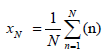 (1)
(1)
This average is then used to calculate a new variable, y(n, N), where:
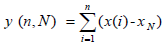 (2)
(2)
The variable y(n, N) is called accumulated departure of the natural record in time [4,6,7,37].
From the accumulated departure y(n, N), the range R(n) is calculated according to the equation [4,6,7,13,37,59,66,67]:
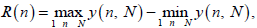 (3)
(3)
R(n) is the distance between the minimum and maximum value of y(n, N).
From the natural time-series, X(n), the standard deviation, S(n), is calculated by:
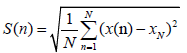 (4)
(4)
The R/S ratio is expected to have a power-law dependence on the bin size
 (5)
(5)
Where H is the Hurst exponent and C is a constant of proportionality.
The logarithmic transformation of equation (5) is a linear equation
 (6)
(6)
From which the Hurst exponent H can be calculated through a least-square fit.
To apply the R/S method the following steps were followed [4]:
i. The signal was divided in segments-windows of certain size (number of samples).
ii. In each segment, the least square fit was applied to the  linear representation of equation (8). Successive representations were considered those exhibiting squares of Spearman’s correlation coefficient above 0.95.
iii. The window was slid for one sample and steps (i)-(ii) were repeated until the end of the signal.
From the above, the time evolution of the Hurst exponent was derived for every signal under investigation.
Hurst exponent estimation through spectral fractal analysis: The complex processes of the preparation of earthquakes evolve naturally in time and space and are associated with characteristic fractal structures [2,3,6,7,11,13,42,43] and references cited in these publications. It is normal to expect that these fractal structures will influence signals derived from the focal area and its vicinity.
The power spectral density, S(f), is the usual method to give helpful information about the intrinsic memory of the system that generates the earthquake [2,3,6,7,13]. Although the power spectrum is only the lowest order statistical measure of the deviations of the random density field from homogeneity, it directly reflects the physical scales of the 1/f processes that govern the structure formation [13].
In the event that a recorded time-series, A(ti), is a temporal fractal, the power spectral density (PSD) is expected to follow a power law, i.e., S (f) = a. f-b, where f is the frequency of the employed transform; for this study, the continuous wavelet transform with base function the Morlet wavelet is employed with f being the central frequency of the Fourier transform that best matches each Morlet scale. The spectral amplification is a measure of the strength of each spectral component in the power spectral density law. On the other hand, the spectral scaling exponent b quantifies the power of the correlations in time or space. The effectiveness of the power-law fit is assessed by the square of the Spearman's correlation coefficient [2,3,6,7]. The most important part, however, is to find and identify noteworthy changes in the scaling exponent prior or during seismic events.
To implement the analysis of fractals on the basis of wavelet-based PSD (hereafter abbreviated as spectral fractal analysis) the following steps were followed:
(i) The MHz EM signals were divided in segments (windows): 1024 samples per segment.
These segmentations were expected to reveal the fractal characteristics of the signals [2,3,6,7,13,54].
(ii) In each segmented portion of the signal the PSD using the Morlet wavelet was calculated and a power-law of the form ofS (f) = a. f-bwas investigated.
(iii) A least square fit was implemented to the log(S (f)) - log (f) transformation of the PSD.
Among the various segments, the successive ones were those with a square of the Spearman's correlation coefficient above 0.95.
(iv) In the successive power-law representations found of step (iii), the Hurst exponents were calculated from the PSD b - values according to the formula pairs [13,29,31]
B = 2.H + 1⇔ H = 0.5. (b - 1) (7)
For the time-series parts following the fractional Brownian motion (fBm) class (1≤ b ≤ 3) and by the formula pairs [12,18,69]
B = 2.H - 1⇔ H = 0.5. (b - 1) (8)
For the time-series parts following the fractional Gaussian noise (fGn) class (-1≤ b < 1).
Note that this implementation is similar to the one described in section 2.2.2. This was done to allow for the direct comparison between the Hurst exponents derived from the R/S analysis with the ones derived from the spectral fractal analysis method and relations (7) and (8) specifically.
Class separation through the R/S and spectral fractal methods: To safely estimate the Hurst exponent in fragmented parts of an EM signal or in its entity, it is important to incorporate the different perspectives that are formulated by the different techniques for the calculation of H. The joined utilisation of different techniques strengthens the identification of the data segments that exhibit long-memory trends. For the correct identification, it is essential to label with reliability the long-memory portions of a time-series, both, through the direct H -calculating technique (R/S) and through the indirect one, namely the spectral fractal analysis. The correct labelling facilitates the precursory marking of the EM segments that can be utilised afterwards for the classification of the long-lasting pre-earthquake signs and also for the right assessment of these. For this situation [68,69] two classes are required, as already implied: (a) The class I segments which comprise the EM time-series sections that can be classified as of noteworthy precursory value (viz., the prominent successive parts, r2 < 0.95, following the fBm class, 1≤ b ≤ 3); (b) The class II segments which consist of EM time-series portions that can be deemed as insignificant or of no earthquake precursory value at all (viz. the segments that do not follow the prominent fBm class, r2 < 0.95 and 1≤ b 3, or are not fBm at all, -1 ≤ b < 1). Obviously, the Class II segments are the complement of the Class I ones [68]. According to several publications, the two longmemory analysis methods that was described in the sections 2.2.2 and 2.2.3, have been evaluated as of having high discrimination significance and for this reason, they were employed here. The problem at hand is to efficiently determine the Class I segments employing both of the long term identifying methods. At first, R/S analysis was employed as a standalone method to search the signal for segments where the Hurst exponent increased significantly. This was based on the findings of previous publications of the reporting team [4,68], where this increase has been characterised as a sign of long-memory and, thus, of high precursory value. Then, both methods were utilised in combination, so as to feed the outcomes of the R/S method with additional information from the spectral fractal method and to correctly mark the prominent (successive fBm) segments against the non-successive fBm or non-fBm segments.
It is important to mention here that, according to the opinion of the authors of this paper, the R/S analysis is a more targeted method for the calculation of the Hurst exponent since it was designed and introduced by [37] precisely for the calculation of this type of exponent. It should be noted though that the discrimination in the fBm and the fGn segments is achieved in principle by the spectral fractal method since it is this method that accounts for the 1/f power-law behaviour of a signal.
Results and Discussion
Figures 4-18 present some characteristic outcomes of the R/S analysis and the spectral fractal method. All the EM signals of these figures were of the MHz range (41 MHz or 46 MHz) and extended one month before the earthquakes of Table 1 and Figure 2. All of these figures present the time evolution of the Hurst exponent within the one-month window of study together with the time series of the associated square of the Spearman’s correlation coefficient (please see also sections 2.2.2 and 2.2.3). The identifiers of the earthquakes are given in Table 1 and the topography is shown in shown in Figures 2 and 3. The days in the presented legends refer to the days of the Julian’s calendar for each indicated year. In the figure caption, JD refers to the term Julian day.

Figure 3: The telemetric network employed for the MHz radiation recordings.

Figure 4: Time evolution of Hurst exponent. (Calculation through sliding-window R/S analysis, EQ: 5, Table 1, Komotini station (Τ), JDs 114-122, 2009, 41 MHz. Time in seconds (a.u.). From top to bottom: the EM signal, the evolution of the Hurst exponent and the time-series of the square of the associated Spearman’s correlation coefficient).

Figure 5: Time evolution of Hurst exponent. (Calculation through sliding-window R/S analysis, EQ: 5, Table 1, Komotini station, JDs 114-122, 2009, 46 MHz. Time in seconds (a.u.). From top to bottom: the EM signal, the evolution of the Hurst exponent and the time-series of the square of the associated Spearman’s correlation coefficient).

Figure 6: Time evolution of Hurst exponent. (Calculation through sliding-window R/S analysis, EQ: 7, Table 1, Ioannina station, JDs 127-150, 2009, 41 MHz. Time in seconds (a.u.). From top to bottom: the EM signal, the evolution of the Hurst exponent and the time-series of the square of the associated Spearman’s correlation coefficient.

Figure 7: Time evolution of Hurst exponent. (Calculation through sliding-window R/S analysis, EQ: 7, Table 1, Ioannina station, JDs 127-150, 2009, 46 MHz. Time in seconds (a.u.). From top to bottom: the EM signal, the evolution of the Hurst exponent and the time-series of the square of the associated Spearman’s correlation coefficient).

Figure 8: Time evolution of Hurst exponent. (Calculation through sliding-window R/S analysis, EQs: 3 and 6, Table 1, Neapoli station, JDs 214-243, 2014, 41 MHz. Time in seconds (a.u.). From top to bottom: the EM signal, the evolution of the Hurst exponent and the time-series of the square of the associated Spearman’s correlation coefficient).

Figure 9: Time evolution of Hurst exponent. (Calculation through sliding-window R/S analysis, EQs: 3 and 6, Table 1, Neapoli station, JDs 214-243, 2014, 46 MHz. Time in seconds (a.u.). From top to bottom: the EM signal, the evolution of the Hurst exponent and the time-series of the square of the associated Spearman’s correlation coefficient).

Figure 10: Time evolution of Hurst exponent. (Calculation through sliding-window R/S analysis, EQ: 1, Table 1, Mytilene station, JDs 114-139, 2014, 41 MHz. Time in seconds (a.u.). From top to bottom: the EM signal, the evolution of the Hurst exponent and the time-series of the square of the associated Spearman’s correlation coefficient).

Figure 11: Time evolution of Hurst exponent. (Calculation through sliding-window R/S analysis, EQ: 1, Table 1, Mytilene station, JDs 114-139, 2014, 46 MHz. Time in seconds (a.u.). From top to bottom: the EM signal, the evolution of the Hurst exponent and the time-series of the square of the associated Spearman’s correlation coefficient).

Figure 12: Box and whiskers plot of the time evolution of the Hurst exponent. (Calculation through R/S analysis, EQ: 1, Table 1, Mytilene station, JDs 114-139, 2014, 41 MHz).

Figure 13: Time evolution of H for fBm segments identified through the spectral fractal method according to the equations (8). (EQ: 2, Table 1, Neapoli station, JDs 152-182, 2009, 41 MHz. Time in seconds. From top to bottom: the evolution of the Hurst exponent, the time-series of the square of the associated Spearman’s correlation coefficient and the EM signal. The blue points indicate successive (r2 < 0.95) fBm segments. The red points refer to the remaining segments. In the legends the mean and the standard deviation of the Hurst exponent and the square of the Spearman’s correlation coefficient is given, as well as the number of the successive fractal segments).

Figure 14: Time evolution of Hurst exponent. (Calculation through sliding-window R/S analysis, EQ: 2, Table 1, Neapoli station, JDs 152-182, 2009, 41 MHz. Time in seconds (a.u.). From top to bottom: the EM signal, the evolution of the Hurst exponent and the time-series of the square of the associated Spearman’s correlation coefficient. The EM signal is identical to the one of Figure 13).

Figure 15: Time evolution of H for fBm segments identified through the spectral fractal method according to the equations (8). (EQ: 2, Table 1, Neapoli station, JDs 152-182, 2009, 46 MHz. Time in seconds. From top to bottom: the evolution of the Hurst exponent, the time-series of the square of the associated Spearman’s correlation coefficient and the EM signal. The blue points indicate successive (r2 < 0.95) fBm segments. The red points refer to the remaining segments. In the legends the mean and the standard deviation of the Hurst exponent and the square of the Spearman’s correlation coefficient is given, as well as the number of the successive fractal segments).

Figure 16: Time evolution of Hurst exponent. (Calculation through sliding-window R/S analysis, EQ: 2, Table 1, Neapoli station, JDs 152-182, 2009, 46 MHz. Time in seconds (a.u.). From top to bottom: the EM signal, the evolution of the Hurst exponent and the time-series of the square of the associated Spearman’s correlation coefficient. The EM signal is identical to the one of Figure 15).

Figure 17: Time evolution of H for fBm segments identified through the spectral fractal method according to the equations (8). (EQ:2, Table 1, Vamos station, JDs 152- 182, 2009, 41 MHz. Time in seconds. From top to bottom: the evolution of the Hurst exponent, the time-series of the square of the associated Spearman’s correlation coefficient and the EM signal. The blue points indicate successive (r2 < 0.95) fBm segments. The red points refer to the remaining segments. In the legends the mean and the standard deviation of the Hurst exponent and the square of the Spearman’s correlation coefficient is given, as well as the number of the successive fractal segments).

Figure 18: Time evolution of Hurst exponent. (Calculation through sliding-window R/S analysis, EQ: 2, Table 1, Vamos station, JDs 152-182, 2009, 41 MHz. Time in seconds (a.u.). From top to bottom: the EM signal, the evolution of the Hurst exponent and the time-series of the square of the associated Spearman’s correlation coefficient. The EM signal is identical to the one of Figure 17).
In reference to the Figures 4-18 the following issues are of significance:
(a) Persistent Hurst exponents were calculated through the R/S analysis for the pre earthquake MHz EM disturbances. The great majority of the calculated H -exponents was in the range 0.7-0.9. Several exponents were above 0.9. This is characteristically shown in the Box and Whiskers plot of Figure 12.
(b) There were several cases where the time-evolution of the Hurst exponent did not follow the one of the EM disturbances. Characteristic cases are shown in Figures 7, 9 and 10. Figure 10 shows this behaviour more characteristically.
(c) In numerous cases, the detected MHz EM disturbances were associated with an increase of the associated Hurst exponent. For example, this can be observed between 0.3 × 10⁶ - 0.5 × 10⁶ s and 0.9 × 10⁶ -1.0 × 10⁶ s in Figure 11. Another characteristic case is shown in Figure 8. In this figure, the Hurst exponents follow, more or less, the EM disturbances after 1.0 × 10⁶ s. The most characteristic case is shown in Figure 6. Note, that an increase in the Hurst exponent has been characterised as a pre-seismic sign of some value.
d) As was systematically observed by the several outcomes of the R/S analysis similar to those of the Figures 1-11 and the Figures 14, 16 and 18, the time profile of the Hurst exponent exhibits small variance when derived by the R/S analysis method. A very characteristic example case is the one of Figure 10. On the other hand, there were also cases where the Hurst exponent evolution of one-month duration presented noteworthy fluctuations. Such are the cases shown in Figures 4, 7 and 8.
(e) The persistent behaviour of the Hurst exponent is identified through the R/S analysis, regardless of the corresponding output of the spectral fractal method. This is characteristically shown in Figure 13 versus Figure 14, in Figure 15 versus Figure 16 and in Figure 17 versus Figure 18. More specifically, as Figures 13, 15 and 17 indicate, the spectral fractal method outlined either a medium anti-persistent behaviour of the EM signal or a rather continuous switching between anti-persistency and persistency. As can be observed from the Figures 13, 15 and 17, all these effects are associated with significant fluctuations. Note, that there are many successive (r2 ≥ 0.95) fBm Class I segments according to the spectral fractal method. Especially, in Figure 17, the profile is mainly fBm. Note also, that the identification of many class I fBm areas prior to earthquakes.
It has been identified as a pre-seismic sign of noteworthy value [5,68]. Despite these findings, the associated Hurst profiles (Figures 14, 16 and 17) are persistent. This persistent behaviour is declared even in the cases with not-successive (r2 < 0.95) segments and/or not fBm ( b∉(1− 3)) Class II segments (red segments of Figures 13, 15 and 17). The issue is related to comment (a) above and is also of importance.
(f) Some H -values derived by the R/S analysis were above 1. This definitely contradicts the theory. To the opinion of the authors, this was due to the statistical errors in estimations of the H - values. Indeed, in order to calculate the Hurst exponent, a least square fit is applied in the log (R) versus log (S) diagram (see also section 2.2.3). In the ± 99% estimation of the corresponding slope, the H -values above 1 were mainly of statistical nature. The statistical errors were not presented in Figures 4-11, as well as, in Figures 13, 15 and 17 to avoid plotting inconsistencies.
The comments (a) and (f) tend to disagree with some findings of the related literature regarding the MHz EM disturbances [11-13,23] and references in these publications. According to these publications, the MHz disturbances show anti-persistent behaviour opposed to the kHz radiation which exhibits persistent fBm profiles (see for example, the reference 23 and the references therein). The persistent behaviour of the kHz radiation has been interpreted, in these publications, as a footprint for the inevitable occurrence of an earthquake. However, related publications mention that there is no one-to one correspondence between earthquakes and anomalies and hence, it is essential to anticipate more related kHz data, regarding the full clarification of this issue. It is also important to note that some interpretations for the Hurst exponent in the above publications were based on the spectral fractal analysis of the signals and the association of H with b according to equations (7) and (8). As indicated in the Figures 13, 15 and 17, the spectral fractal method tends to produce anti-persistent behaviour. Indeed, if one calculates Hurst exponents from the wavelet spectral fractal analysis method then for certain segments, anti-persistent H -profiles are calculated, as this was characteristically shown in Figures 13 versus 14, Figures 15 versus 16 and Figures 17 versus 18. The Hurst exponents of this paper that were calculated by the spectral fractal method, provided similar Hurst exponents for the MHz radiation prior to earthquakes as those already identified by other papers on preseismic EM radiation and also by papers on pre-earthquake time series of radon concentration in soil [2,3,6,7]. It is very significant to note that a very recent report of the authors [68] indicated that, despite the discrepancies in the H -estimations between the spectral fractal method and the R/S analysis, both methods can be combined very efficiently through Support Vector Machine (SVM) classifiers to detect successive fBm segments in MHz EM signals. Two characteristic results are presented in Figures 19 and 20 especially when viewed under the perspective of the corresponding Figures 15 and 17. Indeed, as can be observed from Figures 19 and 20, the time evolution of the successive (r2 ≥ 0.95) fractal fGn segments (-1 ≤ b < 1) is persistent.

Figure 19: Time evolution of H for fGn segments identified through the spectral fractal method according to the equations (8). (EQ: 2, Table 1, Neapoli station, JDs 152-182, 2009, 46 MHz. Time in seconds. From top to bottom: the EM signal, the evolution of the Hurst exponent and the timeseries of the square of the associated Spearman’s correlation coefficient. The EM signal is identical to the one of Figures 13 and 14).

Figure 20: Time evolution of H for fGn segments identified through the spectral fractal method according to the equations (8). (EQ: 2, Table 1, Vamos station, JDs 152-182, 2009, 41 MHz. Time in seconds. From top to bottom: the EM signal, the evolution of the Hurst exponent and the time-series of the square of the associated Spearman’s correlation coefficient. The EM signal is identical to the one of Figures 17 and 18).
From another viewpoint, the deviations in the estimation of H values between the two methods employed in this paper could be due to the fact that in actual situations, there are many processes that act on various scales [2,12,42] and for this reason, the relations b = 2.H + 1 and b = 2.H - 1 potentially do not hold. In general, it may be argued that the H -values calculated from the spectral fractal b-values through equations (7) and (8) are considerably lower and present higher variance. For this reason, the use of the R/S or spectral fractal methods in the estimation of the Hurst exponent should be taken into careful consideration.
From the MHz EM data presented in this paper it becomes evident that the R/S method provides additional information on the estimation of the Hurst exponent when combined with the spectral fractal method. Note that the combined application of both spectral fractal analysis and R/S methods should in principle be applied on the same segments. What is significant however that is the R/S analysis departs from a different mathematical basis as compared to the spectral fractal method. Note that, importantly, the R/S method is considered as the standard method for the calculation of the Hurst exponent. The insight of these new aspects is more characteristically
Supported by two example data, namely those of Figures 21 and 22. These figures (Figures 21 and 22) present a significant new finding; the successive fractal fBm segments of the pre-earthquake MHz signals produce significantly higher Hurst exponents as compared to the ones of the successive fGn segments. What is very important is that this behaviour was systematically validated by several different earthquake data. It is possible that this behaviour allowed the accurate classification of successive fBm versus not successive fBm segments of EM preseismic signals in the above-mentioned recent publication of [68].

Figure 21: Time evolution of Hurst exponent. (EQ: 4, Table 1, Neapoli station, JDs 76-105, 2015, 41 MHz. Successive (blue, r2 ≥ 0.95) fBm ( -1≤ b ≤ 3) segments).

Figure 22: Time evolution of Hurst exponent. (EQ: 4, Table 1, Neapoli station, JDs 76-105, 2015, 41 MHz. Segments not -fBm (-1 ≤ b < 1) and/or segments not-successive (red).
According to the data of Figures 21 and 22, the discussion of [68] and the presented data of this research, it can be supported that the R/S analysis is a very powerful method to trace significant pre-earthquake patterns hidden in pre-seismic time-series, as an increase in H-values of precursory successive (r2 ≥ 0.95) fBm (-1≤ b ≤ 3) segments. This has been supported also in a very recent publication of the author and colleagues [4].
Conclusions
This paper presented the analysis of MHz pre-earthquake signals in terms of the evolution of the Hurst exponent calculated though the R/S analysis and the spectral fractal method. The R/S analysis estimated the Hurst exponent directly while the spectral fractal method, indirectly. From the results presented, several important issues can be summarised:
(1) All the investigated signals exhibited characteristic epochs with fractal organisation (successive fBm segments). In some cases these epochs were continuous and in other cases scattered. Signals with scattered or continuous such epochs have been identified as precursory. Signals with no such epochs have been associated with low seismicity periods.
(2) According to the R/S method several successive fBm segments exhibited persistency. Switching between persistency and antipersistency was also found. Although several references suggested that the MHz EM precursors show only anti-persistent behaviour, the findings of this research supported a different view. The EM MHz disturbances can be either anti-persistent or persistent. The R/S analysis provided mainly persistent behaviour. It is significant that the switching between persistency and anti-persistency has been characterised as a pre-earthquake pattern.
(3) The investigated earthquakes were associated with Hurst warnings up to one month prior to each event. The main batch of the investigated MHz signals gave alarms usually 2-3 weeks and 1 week prior to the earthquake event according to the spectral fractal method. It was concluded that to identify pre-earthquake signs of enhanced significant value, the following steps should be followed:
(a) Employ spectral fractal methods for identifying the successive fBm segments, because these are considered to be associated with longmemory dynamics. These methods can also screen the random fGn segments. Note, that despite the fact that this method is indirect for the estimation of the Hurst exponent, it is the most robust method for the identification of the fBm segments which are of noteworthy precursory value.
(b) After the first screening with spectral fractal analysis, a second screening is applied to identify the segments which are well away from randomness. According to the view of the author this is implemented for successive fBm segments with b > 1.5 or H > 0.25. Other investigators suggest that this is implemented for successive fBm segments with b > 2 or H > 0.5.
(c) A third screening is the application of the R/S analysis, on the same segments of (a). If the strong fBm (high b -exponent) segments are associated with an increase in H - values from the R/S analysis, then the precursory value is enhanced.
The final conclusion of this research is that, more or less, both techniques should be employed in steps, where the power-law spectral fractal analysis is the most significant technique to trace long memory patterns of 1/f processes as those in earthquake preparation, while the R/S method is the direct and more robust method for the estimation of the Hurst exponent.
References
- Petraki E, Nikolopoulos D, Nomicos C, Stonham J, Cantzos D, et al. (2015) Electromagneticpre-earthquake precursors: Mechanisms, data and models-A review. J Earth SciClim Change 6: 1-11.
- Nikolopoulos D, Petraki E, Marousaki A, Potirakis S, Koulouras G, et al. (2012) Environmental monitoring of radon in soil during a very seismically active period occurred in South West Greece. J Environ Monitor 14: 564-578.
- Nikolopoulos D, Petraki E, Vogiannis E, Chaldeos Y, Giannakopoulos P, et al.(2014) Traces of self-organisation and long-range memory in variations of environmental radon in soil: Comparative results from monitoring in Lesvos Island and Ileia (Greece). J RadioanalNuclCh 299: 203-219.
- Nikolopoulos D, Petraki E, Nomicos C, Koulouras G, Kottou S, et al. (2015) Long-memory trends in disturbances of radon in soil prior ML=5.1 earthquakes of 17 November2014, Greece. J Earth SciClim Change 6: 1-11.
- Petraki E (2016) Electromagnetic radiation and radon-222 Gas emissions as precursors of seismic activity. A thesis submitted for the degreeof Doctor of Philosophy, Department of Electronic and Computer Engineering, Brunel University London, UK.
- Petraki E, Nikolopoulos D, Fotopoulos A, Panagiotaras D, Koulouras G, et al.(2013) Self-organised critical features in soil radon and MHz electromagnetic disturbances: Results from environmental monitoring in Greece. ApplRadiat Isotopes 72: 39–53.
- Petraki E, Nikolopoulos D, Fotopoulos A, Panagiotaras D, Nomicos C, et al. (2013) Long-range memory patterns in variations of environmental radon in soil. Anal Methods 5: 4010-4020.
- Khan PA, Tripathi SC, Mansoori AA, Bhawre P, Purohit PK, et al. (2011) Scientific efforts in the direction of successful earthquake prediction. IJGGS 1: 669-677.
- Keilis-Borok VI, Soloviev AA (2003) Nonlineardynamics of the lithosphere and earthquake prediction. Heidelberg: Springer.
- Hayakawa M, Hobara Y (2010) Current status of seismo-electromagnetics for short-term earthquake prediction. Geomat Nat Haz Risk 1: 115-155.
- Eftaxias K, Balasis G, Contoyiannis Y, Papadimitriou C, Kalimeri M, et al. (2010) Unfolding the procedure of characterizing recorded ultra low frequency, kHZ and MHz electromagnetic anomalies prior to the L’Aquila earthquake as pre-seismic ones - Part 2. NHESS 10: 275–294.
- Eftaxias K (2010) Footprints of non-extensive Tsallis statistics, self-affinity and universality in the preparation of the L'Aquila earthquake hidden in a pre-seismic EM emission. Physica A 389: 133-140.
- Eftaxias K, Athanasopoulou L, Balasis G, Kalimeri M, Nikolopoulos S, et al. (2009) Unfolding the procedure of characterizing recorded ultra low frequency, kHz and MHz electromagnetic anomalies prior to the L’Aquila earthquake as pre-seismic ones – Part 1. NHESS 9: 1953-1971.
- Balasis G, Daglis I, Papadimitriou C, Kalimeri M, Anastasiadis A, et al. (2008) Dynamical complexity in DST time series using non-extensive Tsallis entropy. Geophys Res Lett 35: L14102.
- Balasis G, Daglis IA, Papadimitriou C, Kalimeri M, Anastasiadis A, et al. (2009) Investigating dynamical complexity in the magnetosphere using various entropy measures. J Geophys Res 114: A00D06.
- Balasis G, Mandea M (2007) Can electromagnetic disturbances related to the recent great earthquakes be detected by satellite magnetometers? Tectonophysics 431: 173–195.
- Contoyiannis YF, Diakonos FK, Kapiris PG, Peratzakis AS, Eftaxias KA (2004) Intermittent dynamics of critical pre-seismic electromagnetic fluctuations. PhysChem Earth 29: 397- 408.
- Contoyiannis Y, Kapiris P, Eftaxias K (2005) Monitoring of a pre-seismic phase from its electromagnetic precursors. Phys Rev E 71: 066123.
- Contoyiannis YF, Eftaxias K (2008) Tsallis and levy statistics in the preparation of an earthquake. Nonlinear Process Geophys 15: 379–388.
- Eftaxias K, Kapiris P, Polygiannakis J, Bogris N, Kopanas J, et al. (2001) Signature of pending earthquake from electromagnetic anomalies. Geophys Res Lett 29: 3321–3324.
- Eftaxias K, Kapiris P, Dologlou E, Kopanas J, Bogris N, et al. (2002) EM anomalies before the Kozani earthquake: a study of their behavior through laboratory experiments. Geophys Res Lett 29: 69-1–69-4.
- Eftaxias K, Kapiris P, Balasis G, Peratzakis A, Karamanos K, et al. (2006) Unified approach to catastrophic events: from the normal state to geological or biological shock in terms of spectral fractal and nonlinear analysis. NHESS 6: 205-228.
- Eftaxias K, Contoyiannis Y, Balasis G, Karamanos K, Kopanas J, et al. (2008) Evidence of fractional-Brownian-motion-type asperity model for earthquake generation in candidate pre-seismic electromagnetic emissions. NHESS 8: 657-669.
- Eftaxias K, Panin V, Deryugin Y (2007) Evolution-EM signals before earthquakes in terms of meso-mechanics and complexity. Tectonophysics 431: 273–300.
- Hadjicontis V, Mavromatou C, Eftaxias K (2002) Pre-seismic earth’s field anomalies recorded at Lesvos station, North-Eastern Aegean. AcGeP 50: 151-158.
- Kalimeri M, Papadimitriou C, Balasis G, Eftaxias K (2008) Dynamical complexity detection in pre-seismic emissions using non-additive Tsallis entropy. Physica A 387: 1161-1172.
- Kapiris P, Balasis G, Kopanas J, Antonopoulos G, Peratzakis A, et al. (2004) Scaling similarities of multiple fracturing of solid materials. Nonlinear Process Geophys 11: 137–151.
- Kapiris PG, Eftaxias KA, Chelidze TL (2004) Electromagnetic signature of prefracture criticality in heterogeneous media. Phys Rev Lett 92: 065702-1/065702-4.
- Kapiris PG, Eftaxias KA, Nomikos KD, Polygiannakis J, Dologlou E, et al. (2003) Evolving towards a critical point: A possible electromagnetic way in which the critical regime is reached as the rupture approaches. Nonlinear Process Geophys 10: 511–524.
- Kapiris P, Nomicos K, Antonopoulos G, Polygiannakis J , Karamanos K, et al. (2005) Distinguished seismological and electromagnetic features of the impending global failure: Did the 7/9/1999 M5.9 Athens earthquake come with a warning? Earth Planets Space 57: 215–230.
- Kapiris P, Polygiannakis J, Peratzakis A, Nomicos K, Eftaxias K (2002) VHF-electromagnetic evidence of the underlying pre-seismic critical stage. Earth Planets Space 54: e1237–e1246.
- Karamanos K (2001) Entropy analysis of substitutive sequences revisited. J Phys A 34: 9231-9241.
- Karamanos K, Nicolis G (1999) Symbolic dynamics and entropy analysis of Feigenbaum limit sets. Chaos, Solitons Fractals 10: 1135-1150.
- Karamanos K, Peratzakis A, Kapiris P, Nikolopoulos S, Kopanas J, et al. (2005) Extractingreseismic electromagnetic signatures in terms of symbolic dynamics. Nonlinear Process Geophys 12: 835–848.
- Cicerone R, Ebel J, Britton J (2009) A systematic compilation of earthquake precursors. Tectonophysics 476: 371-396.
- Nomicos K, Vallianatos F (1998) Electromagnetic variations associated with the seismicity of the frontal Hellenic arc. GeolCarpath 49: 57-60.
- Hurst H (1951) Long term storage capacity of reservoirs. T Am SocCivEng 116: 770-799.
- Hurst H, Black R, Simaiki Y (1965) Long-term storage: an experimental study. London: Constable.
- Koulouras G, Kontakos K, Stavrakas I, Stonham J, Nomicos K (2005) Embedded compact flash. IEEE Circuits Device 21: 27-34.
- Shrivastava A (2014) Are pre-seismic ULF electromagnetic emissions considered as a reliable diagnostics for earthquake prediction? CurrSci 107: 596-600.
- Uyeda S, Nagao T, Kamogawa M (2009) Short-term earthquake prediction: current status of seismo- lectromagnetics. Tectonophysics 470: 205–213.
- Smirnova NA, Hayakawa M (2007) Fractal characteristics of the ground-observed ULF emissions in relation to geomagnetic and seismic activities. J Atmos Sol TerrPhys 69: 1833-1841.
- Smirnova N, Hayakawa M, Gotoh K (2004) Precursory behavior of fractal characteristics of the ULF electromagnetic fields in seismic active zones before strong earthquakes. PhysChem Earth 29: 445-451.
- Yonaiguchi N, Ida Y, Hayakawa M, Masuda S (2007) Fractal analysis for VHF electromagnetic noises and the identification of pre-seismic signature of an earthquake. J Atmos Sol TerrPhys 69: 1825-1832.
- Fraser-Smith AC, Bernardi A, McGill PR, Ladd ME, Helliwell RA, et al. (1990) Lowfrequency magnetic field measurements near the epicenter of the Ms 7.1 Loma Prieta earthquake. Geophys Res Lett 17: 1465-1468.
- Fujinawa Y, Takahashi K (1998) Electromagnetic radiations associated with major earthquakes. Phys Earth Planet Inter 105: 249-259.
- Hayakawa M, Ida Y, Gotoh K (2005) Multifractal analysis for the ULF geomagnetic data duringthe Guam earthquake. Electromagnetic Compatibility and Electromagnetic Ecology, 2005. IEEE 6th International Symposium 11: 239 – 243.
- Kopytenko Yu A, Matiashviali TG, Voronov PM, Kopytenko EA, Molchanov OA (1993) Detection of ultra-low-frequency emissions connected with the Spitak earthquake and its aftershock activity, based on geomagnetic pulsations data at Dusheti and Vardzia observatories. Phys Earth Planet Inter 77: 85-95.
- Smith B, Johnston M (1976) Atectonomagnetic effect observed before a magnitude 5.2 earthquake near Hollister, California. J Geophys Res 81: 3556-3560.
- Enomoto Y, Tsutsumi A, Fujinawa Y, Kasahara M, Hashimoto H (1997) Candidate precursors: pulse-like geo-electric signals possibly related to recent seismic activity in Japan. Geophys J Int 131: 485-494.
- Maeda K, Tokimasa N (1996) Decametric radiation at the time of the Hyogo-ken Nanbu earthquake near Kobe in 1995. Geophys Res Lett 23: 2433-2436.
- Varotsos P, Sarlis N, Eftaxias K, Lazaridou M, Bogris N, et al. (1999) Prediction of the 6.6 Grevena-Kozani Earthquake of May 13, 1995. PhysChem Earth 24: 115-121.
- Warwick J, Stoker C, Meyer T (1982) Radio emission associated with rock fracture: Possible application to the Great Chilean Earthquake of May 22, 1960. J Geophys Res 87: 2851-2859.
- Petraki E, Nikolopoulos D, Chaldeos Y, Coulouras G, Nomicos C, et al.(2014) Fractal evolution of MHz electromagnetic signals prior to earthquakes: results collected in Greece during 2009. Geomat Nat Haz Risk 7: 550-564.
- Minadakis G, Potirakis S, Nomicos C, Eftaxias K (2012) Linking electromagnetic precursors with earthquake dynamics: An approach based on non-extensive fragment and self-affine asperity models. Physica A 391: 2232–2244.
- Potirakis SM, Minadakis G, Nomicos C, Eftaxias K (2011) A multidisciplinary analysis for traces of the last state of earthquake generation in preseismic electromagnetic emissions. NHESS 11: 2859–2879.
- Potirakis S, Minadakis G, Eftaxias K (2012) Analysis of electromagnetic pre-seismic emissions using Fisher information and Tsallis entropy. Physica A 391: 300-306.
- Potirakis SM, Minadakis G, Eftaxias K (2013) Relation between seismicity and pre-earthquakeelectromagnetic emissions in terms of energy, information and entropy content. NHE 12: 1179-1183.
- Lopez T, Mart�?±nez-Gonzalez C, Manjarrez J, Plascencia N, Balankin A (2009) Fractal Analysis of EEG Signals in the Brain of Epileptic Rats, with and without Biocompatible Implanted Neuroreservoirs. AMM 15: 127-136.
- Rehman S, Siddiqi A (2009) Wavelet based Hurst exponent and fractal dimensional analysis of Saudi climatic dynamics. Chaos Solitons Fractals 39: 1081-1090.
- Gilmore M, Yu C, Rhodes T, Peebles W (2002) Investigation of rescaled range analysis, the Hurst exponent, and long-time correlations in plasma turbulence. Phys Plasmas 9: 1312-1317.
- Kilcik A, Anderson C, Rozelot J, Ye H, Sugihara G, et al. (2009) Non-linear prediction of solar cycle 24. Astrophys J 693: 1173–1177.
- Li X, Polygiannakis J, Kapiris P, Peratzakis A, Eftaxias K, et al. (2005) Fractal spectral analysis of pre-epileptic seizures in terms of criticality. J Neural Eng 2: 11-6.
- Granero MS, Segovia JT, Perez JG (2008) Some comments on Hurst exponent and the long memory processes on capital markets. Physica A 387: 5543–5551.
- Dattatreya G (2005) Hurst parameter estimation from noisy observations of data traffic traces. Paper presented at the 4th WSEAS International Conference on Electronics, Control and Signal Processing, Miami, Florida, USA, p: 193–198.
- Stratakos J, Sakellariou M (2006) Anevaluation of methods for the estimation of the fractal dimension of rock surfaces. Technical Chron. Science Journal, I, No 1–2.
- Wawszczak J (2005) Methods for estimating the Hurst exponent. The analysis of its value for fracture surface research. Mater Sci-Poland 23: 585-590.
- Cantzos D, Nikolopoulos D, Petraki E, Nomicos C, Yannakopoulos PH, et al. (2015) Identifying long-memory trends in pre-seismic MHz disturbances through support vector machines. J Earth SciClim Change 6: 1-9.
- Buldyrev S, Goldberger A, Havlin S, Manligna R, Matsa M, et al. (1995) Long-range correlations properties of coding and non-coding DNA sequences: GenBank analysis. Phys Rev E Stat Phys Plasmas Fluids RelatInterdiscip Topics 51: 5084-5091.
Relevant Topics
- Atmosphere
- Atmospheric Chemistry
- Atmospheric inversions
- Biosphere
- Chemical Oceanography
- Climate Modeling
- Crystallography
- Disaster Science
- Earth Science
- Ecology
- Environmental Degradation
- Gemology
- Geochemistry
- Geochronology
- Geomicrobiology
- Geomorphology
- Geosciences
- Geostatistics
- Glaciology
- Microplastic Pollution
- Mineralogy
- Soil Erosion and Land Degradation
Recommended Journals
Article Tools
Article Usage
- Total views: 12496
- [From(publication date):
July-2016 - Jul 16, 2025] - Breakdown by view type
- HTML page views : 11503
- PDF downloads : 993