Studies on Genetic Diversity in Upland Rice (Oryza sativa L.) Genotypes Evaluated at Gojeb and Guraferda, Southwest Ethiopia
Received: 24-Jul-2019 / Manuscript No. ACST-23-577 / Editor assigned: 29-Jul-2019 / PreQC No. ACST-23-577(PQ) / Reviewed: 12-Aug-2019 / QC No. ACST-23-577 / Revised: 15-Jun-2023 / Manuscript No. ACST-23-577(R) / Published Date: 13-Jul-2023 QI No. / ACST-23-577
Abstract
The study was conducted using thirty six upland rice genotypes during the 2017 main rainy season at two experimental sites of Bonga agricultural research center; southwestern Ethiopia to classify and identify groups of similar genotypes and thereby estimate the genetic difference between clusters of the genotypes, the experiment was laid down in 6 × 6 simple lattice design. The combined analysis of variance over the two locations revealed that the genotypes showed highly significant (P ≤ 0.01) differences for all the characters studied, except for days to 50% heading, panicle weight, thousand seed weight, lodging incidences, leaf blast and brown spot. Similarly genotype × location interactions revealed highly significant (P ≤ 0.01) differences for panicle shattering and grain yield and significant (P ≤ 0.05) differences for days to 85% maturity, plant height, number of fertile tillers per plant, number of unfilled spikelets per panicle and biomass yield. The squared distance (D2) analysis grouped the 36 genotypes in to four clusters. This makes the genotypes become moderately divergent. The chi-square (x2) test showed that all inter-cluster squared distances was highly significant. The principal component analysis revealed that four principal components have accounted for 70.54% of the total variation.
Keywords
Upland rice; Genetic diversity; Cluster analysis; Principal component analysis
Introduction
Rice belongs to the genus Oryza within the grass family Gramineae (Poaceae). There are about 25 species of Oryza. Of these only two species are cultivated, namely Oryza sativa and Oryza glaberrima. Rice (Oryza sativa L.) is the most important food crop and energy source for about half of the world’s population. More than 3.5 billion people in the world depend on rice for more than 20% of their daily calories. Rice (Oryza sativa L.) is grown in more than 117 countries across all habitable continents covering a total area of about 163 million hectares with a global production of about 740 million metric tons. Asia is the leader in rice production accounting for about 90% of the world's production. Over 75% of the world supply is consumed by people in Asian countries and thus, rice is of immense importance to food security of Asia [1].
Rice is also an important staple food crop in many African countries. It is largely cultivated in West Africa. It has been the most rapidly growing food source across the continent. However, the local production is largely insufficient to meet the consumption needs. Annual rice production in Sub-Saharan Africa (SSA) is estimated to be 14.5 million metric tons. Most of this rice is produced by smallholder farmers. In contrast, Africa‘s rice consumption is about 21 million metric tons creating a deficit of about 6.5 million metric tons per year valued at US $1.7 billion that is imported annually. Overall, imported rice accounts for roughly 31 percent of Sub-Saharan Africa local rice consumption [2]. Cultivation of rice in Ethiopia is a recent phenomenon it was started first at Fogera and Gambella plains in the early 1970’s and grown under widely varying conditions of altitude and climate. It is important cereal crop cultivated in different parts of the country next to teff, maize, wheat and sorghum. Considering the importance and potential of the crop, it has been recognized by the government as the new millennium crop of Ethiopia to attain food security [3].
The potential area for rice production in Ethiopia is estimated to be about 30 million hectares (5 million hectares highly suitable and about 25 million hectares suitable). According to CSA the average rice productivity in Ethiopia is about 2.8 t ha-1, which is much lower than that of the world’s average (4.4 t ha-1). This low productivity of rice in Ethiopia is attributed to a number of factors such as shortage of improved varieties, lack of recommended crop management practices, lack of pre- and post-harvest management technologies and lack of awareness on its utilization [4].
One of the most important approaches to rice breeding is hybridization. Parents choice is the first step in plant breeding program through hybridization. Genetic diversity is the most important tool for plant breeder in choosing the right type of parents for hybridization programme. The divergence can be studied by using technique D2 statistics developed by mahalanobis. Estimation of genetic diversity is also an important factor to know the source of genes for a particular trait within the available genotypes [5]. Appropriate selection of the parents is essential to be used in crossing nurseries to enhance the genetic recombination for potential yield increase. Principal component analysis helps researchers to distinguish significant relationship between traits. This is a multivariate analysis method that aims to explain the correlation between a large set of variables in terms of a small number of underlying independent factors. The main objective of this study is to estimate the magnitude of genetic divergence present in the 36 upland rice genotypes by using cluster analysis and cluster analysis-PCA-based methods for selection of parents in hybridization programme [6].
Materials And Methods
Description of the experimental sites
The experiment was conducted during the main rainy season of 2017 in two locations namely, Gojeb and Guraferda, Southwestern Ethiopia. Gojeb experimental site is located in Kaffa zone of Southern Nations, Nationalities and Peoples Region (SNNPR), which is located 439 km away from Southwest of Addis Ababa [7]. Geographically, Gojeb experimental site is situated at 07°15'0'' N latitude and 036°0'0'' E longitude with an altitude of 1235 m.a.s.l. Its average annual rainfall is 1710 mm with minimum and maximum temperatures of 16.7°C and 24°C, respectively. The soil type of Gojeb is volcanic origin and is classified as the andosol orders with clay loam texture. Guraferda experimental site is also located in Bench Maji zone of Southern Nations, Nationalities and Peoples Region (SNNPR), which is located 590 km away from Southwest of Addis Ababa. Guraferda experimental site is situated at 06°50'368" N latitude and 035°17'16" E longitude with an altitude of 1138 m.a.s.l. The annual average temperatures range from 25°C to 39°C. The area receives maximum rainfall from June to September and the amount ranges between 1200 mm to 1332 mm per annum. The soil type of Guraferda is in the acrisol orders with sandy clay loam texture [8].
Experimental materials
In this experiment, 33 upland rice genotypes, obtained from two different sets of variety trials conducted by rice breeding section of Fogera National Rice Research and Training Center (FNRRTC) and three released varieties (NERICA-12, NERICA-4 and Adet), a total of 36 upland rice genotypes were used (Table 1) [9].
| No | Genotypes | Status | Seed source | Origin |
|---|---|---|---|---|
| 1 | ART15 8-10-36-4-1-1-B-B-1 | 2016/17 PVT | FNRRTC | Africa rice center |
| 2 | ART15 10-17-46-2-2-2-B-B-2 | 2016/17 PVT | FNRRTC | Africa rice center |
| 3 | ART16 9-16-21-1-B-2-B-B-1 | 2016/17 PVT | FNRRTC | Africa rice center |
| 4 | ART16 9-29-10-2-B-1-B-B-1 | 2016/17 PVT | FNRRTC | Africa rice center |
| 5 | ART16-4-1-21-2-B-2-B-1-1 | 2016/17 PVT | FNRRTC | Africa rice center |
| 6 | ART16-4-13-1-2-1-1-B-1-1 | 2016/17 PVT | FNRRTC | Africa rice center |
| 7 | ART16-5-10-2-3-B-1-B-1-2 | 2016/17 PVT | FNRRTC | Africa rice center |
| 8 | ART16-9-1-9-2-1-1-B-1-1 | 2016/17 PVT | FNRRTC | Africa rice center |
| 9 | ART16-9-4-18-4-2-1-B-1-1 | 2016/17 PVT | FNRRTC | Africa rice center |
| 10 | ART16-9-4-18-4-2-1-B-1-2 | 2016/17 PVT | FNRRTC | Africa rice center |
| 11 | ART16-9-6-18-1-1-2-B-1-1 | 2016/17 PVT | FNRRTC | Africa rice center |
| 12 | ART16-9-9-25-2-1-1-B-2-1 | 2016/17 PVT | FNRRTC | Africa rice center |
| 13 | ART16-9-9-25-2-1-1-B-2-2 | 2016/17 PVT | FNRRTC | Africa rice center |
| 14 | ART16-9-29-16-1-1-1-B-1-1 | 2016/17 PVT | FNRRTC | Africa rice center |
| 15 | ART16 15-10-1-1-B-1-B-B-1 | 2016/17 PVT | FNRRTC | Africa rice center |
| 16 | ART16 15-10-1-1-B-1-B-B-2 | 2016/17 PVT | FNRRTC | Africa rice center |
| 17 | ART16-13-11-1-2-B-2-B-2-1 | 2016/17 PVT | FNRRTC | Africa rice center |
| 18 | ART16-16-1-14-3-1-1-B-1-2 | 2016/17 PVT | FNRRTC | Africa rice center |
| 19 | ART16-16-11-25-1-B-1-B-1-2 | 2016/17 PVT | FNRRTC | Africa rice center |
| 20 | ART16-17-7-18-1-B-1-B-1-1 | 2016/17 PVT | FNRRTC | Africa rice center |
| 21 | ART16-21-5-12-3-1-1-B-2-1 | 2016/17 PVT | FNRRTC | Africa rice center |
| 22 | ART16-9-29-12-1-1-2-B-1-1 | 2016/17 NVT | FNRRTC | Africa rice center |
| 23 | ART16-9-14-16-2-2-1-B-1-2 | 2016/17 NVT | FNRRTC | Africa rice center |
| 24 | ART16-9-33-2-1-1-1-B-1-2 | 2016/17 NVT | FNRRTC | Africa rice center |
| 25 | ART16-9-122-33-2-1-1-B-1-1 | 2016/17 NVT | FNRRTC | Africa rice center |
| 26 | ART15-19-5-4-1-1-1-B-1-1 | 2016/17 NVT | FNRRTC | Africa rice center |
| 27 | ART16-5-9-22-2-1-1-B-1-2 | 2016/17 NVT | FNRRTC | Africa rice center |
| 28 | ART16-21-4-7-2-2-2-B-2-2 | 2016/17 NVT | FNRRTC | Africa rice center |
| 29 | ART16-9-16-21-1-2-1-B-1-1 | 2016/17 NVT | FNRRTC | Africa rice center |
| 30 | ART15-13-2-2-2-1-1-B-1-2 | 2016/17 NVT | FNRRTC | Africa rice center |
| 31 | ART15-16-45-1-B-1-1-B-1-2 | 2016/17 NVT | FNRRTC | Africa rice center |
| 32 | ART16-5-10-2-3-B-1-B-1-1 | 2016/17 NVT | FNRRTC | Africa rice center |
| 33 | ART16-4-1-21-2-B-2-B-1-2 | 2016/17 NVT | FNRRTC | Africa rice center |
| 34 | NERICA-12 | Released variety | FNRRTC | Africa rice center |
| 35 | NERICA-4 | Released variety | FNRRTC | Africa rice center |
| 36 | Adet | Released variety | FNRRTC | Africa rice center |
Note: PVT=Preliminary Variety Trial; NVT=National Variety Trial; FNRRTC=Fogera National Rice Research and Training Center
Table 1: Description of the experimental materials.
Experimental design and trial management
The field experiment was laid down in 6 × 6 simple lattice design. The gross plot size of the experiment was 7 m2 (4 m long and 1.75 m wide) each and there were seven rows at 0.25 m interval. The net (harvestable) plot size of the experiment was 5 m2 (4 m length and 1.25 m wide) each. There were a 0.35 m, 0.6 m and 1 m distance between plots, incomplete blocks and replications, respectively [10]. Fertilizer was applied at a rate of 100 kg ha-1 DAP and 100 kg ha-1 as per national recommendation. All DAP was applied during planting while, urea was applied in three splits, with one third at planting, one third at tillering and the remaining one third at panicle initiation. The seeds were drilled in rows with seed rate of 60 kg ha-1. Hand weeding was used for weed control and all other agronomic practices were done uniformly [11].
Data collected
Based on the standard evaluation system for rice developed by International Rice Research Institute (IRRI), 2013 and biodiversity international, 2007 the following eighteen yield and yield related traits were collected from the central five rows of each plot.
Plant height: The height of five randomly taken plants were measured at harvest maturity from the ground level to the tip of the tallest panicle in centimeter and averaged.
Panicle length: The panicle of five randomly taken plants were measured at harvest maturity from the first panicle branch starts to the tip of the panicle in centimeter and averaged.
Number of total tillers per plant: The number of total tillers per plant were counted from five randomly taken plants at booting stage and averaged.
Number of fertile tillers per plant: The number of fertile tillers per plant were counted from five randomly taken plants at harvest maturity and averaged.
Number of filled spikelets per panicle: The numbers of filled spikelets per panicle were counted from five main panicles of five randomly taken plants at harvest maturity and averaged.
Number of unfilled spikelets per panicle: The number of unfilled spikelets per panicle were counted from five main panicles of five randomly taken plants at harvest maturity and averaged.
Panicle weight: Five main panicles from five randomly taken plants were harvested and weighed in gram at harvesting.
Disease severity: Leaf blast and brown spot infections were visually scored on 0-9 scale at heading stage where, 0 was no disease observed and 9 was >75% leaf area affected.
Days to 50% heading: The number of days from the date of emergency up to the date when the tips of the panicle first emerged from the main shoots on 50% of the plants in a plot.
Days to 85% maturity: The number of days from the date of emergency to the date when 85% of grains on panicle are matured.
Number of panicles per meter square: The number of panicles were counted by random draw of 0.25 m2 quadrant (0.5 m × 0.5 m) in the center of each plot.
Harvest index: It is the ratio of grain yield per plot in gram to biomass yield per plot expressed in percent at harvest maturity.
Thousand seed weight: The weight of 1000 seeds in gram from bulked seeds were measured and adjusted at 14% seed moisture basis.
Panicle shattering: The extent to which seeds have shattered from the panicle was visually scored on 1-9 scale at harvest maturity where, 1 ≤ 1% and 9 ≥ 50%.
Lodging incidence: A percentage of plants that are lodged were scored visually on a 1-9 point scale at maturity where 1 was no lodging and 9 were totally lodged.
Grain yield: Taken by weighing grain yield in gram obtained from five central rows in each plot and converted into kilogram per hectare at 14% moisture content.
Statistical analysis
Analysis of variance: To compute a combined statistical analysis across locations, test of homogeneity of error variances of each character for the two locations were performed by using F-max test method of Hartley, which is based on the ratio of the largest mean square of error to the smallest mean square of error. The F-max test showed all characters met the homogeneity assumption. Then all the characters were subjected to pooled analysis of variance over locations using the SAS (v 9.3) mean separation among treatment means were done by using LSD at 5% probability level [12].
Multivariate analysis
Cluster analysis: Clustering was performed using the proc cluster procedure of SAS version 9.3 by employing the method of average linkage clustering strategy of the observation. The number of cluster was determined by following the approach suggested by copper and milligan by looking into three statistics namely pseudo F, pseudo t2 and cubic clustering criteria. The points where local peaks of the CCC and pseudo F-statistic join with small values of the pseudo-t2 statistic followed by a larger pseudo-t2 for the next cluster combination was used to determine the number of clusters. The dendrogram was constructed by using minitab 14 software package based on the average linkage and mahalanobis used as a measure of dissimilarity (the distance) technique [13].
Genetic divergence analysis
Genetic divergence between clusters was determined using the generalized mahalanobis D2 statistics (mahalanobis) using the equation. In matrix notation, the distance between any two groups was estimated from the following relationship.
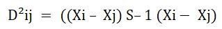
Where: D²ij=The squared distance between any two genotypes i and j
Xi and Xj=The vectors of the values for ith and jth genotypes, respectively
S-1=The inverse of the pooled covariance matrix with in groups
The D2 values obtained for pairs of clusters were considered as the calculated values of chi-square (X2) and tested against tabulated X2 values at n-1 degree of freedom at 1% and 5% probability levels, where n=number of characters considered.
Principal component analysis
Principal component analysis was computed using correlation matrix of SAS version 9.3 in order to examine the relationships among the quantitative characters that are correlated among each other by converting into uncorrelated characters called principal components. Below is the general formula to compute scores on the first component extracted (created) in a principal component analysis [14].
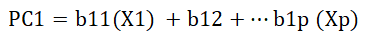
Where: PC1=The subject’s score on principal component 1 (the first component extracted)
b1p=The regression coefficient (or weight) for observed variable p, as used in creating principal component 1
Xp=the subject’s score on observed variable p
Results And Discussion
Analysis of variance
The combined Analyses of Variance (ANOVA) for different characters are presented in Table 2. The combined analysis of variance revealed significant differences among the rice genotypes for all the characters studied, except for days to 50% heading, panicle weight, thousand seed weight, lodging incidence, leaf blast and brown spot, indicates the presence of variation among the tested rice genotypes.
Reported significant differences among 36 rice genotypes for biomass yield, days to maturity, filled grains per panicle, fertile tillers per plant, grain yield, harvest index, plant height, panicle length and unfilled grains per panicle. Reported significant differences among 14 upland rice genotypes for days to maturity, plant height, panicle length and grain yield per hectare. Also reported significant difference among genotypes for days to maturity, panicles per meter square, plant height and grain yield [15].
The mean squares due to genotype × location interactions were differed significantly for panicle shattering, grain yield (kg ha-1), days to 85% maturity, plant height, fertile tillers per plant, unfilled spikelets per panicle and biomass yield. This significant difference of genotype × location interactions indicates differential response of genotypes to the two locations for these characters.
Founds significant genotype × location interaction effects for days to maturity, plant height and grain yield. Also reported significant genotype × location interaction effects for biomass yield, days to maturity, fertile tillers per plant, plant height, panicle length and grain yield.
| Characters | MSL | MSG | MSG×L | MSE | CV |
|---|---|---|---|---|---|
| DH | 15.34ns | 9.55ns | 7.01ns | 6.1 | 3.04 |
| DM | 108.51** | 22.61** | 13.91* | 8.29 | 2.46 |
| PH | 190.44** | 79.67** | 19.72* | 11.75 | 4.11 |
| PL | 0.75ns | 2.98** | 1.51ns | 1.08 | 4.82 |
| TTPP | 26.52** | 6.14** | 2.67ns | 2.61 | 13.21 |
| FTPP | 18.20** | 6.11** | 3.67* | 2.09 | 14.97 |
| FSPP | 123.58ns | 324.73** | 165.40ns | 155.29 | 12.73 |
| USPP | 27.04** | 5.74** | 3.96* | 2.33 | 13.78 |
| PW | 15.80** | 2.56ns | 1.82ns | 1.76 | 8.78 |
| Pan/m2 | 30.25ns | 120.29** | 47.55ns | 44.95 | 14.36 |
| BY | 4033402.78** | 1128445.63** | 686545.63* | 413372.2 | 15.68 |
| HI | 0.0001ns | 0.0067** | 0.0036ns | 0.0027 | 14.64 |
| TSW | 55.95** | 10.48ns | 7.06ns | 6.68 | 9.06 |
| +LB | 11.61ns | 26.55ns | 25.02ns | 16.78 | 19.13 |
| +BS | 72.35* | 24.90ns | 21.97ns | 16.27 | 15.08 |
| $LI | 0.001ns | 0.50ns | 0.42ns | 0.32 | 20.1 |
| $PSht | 0.92ns | 2.47** | 2.12** | 0.29 | 22.71 |
| GY | 1898539.52** | 288979.76** | 226956.50** | 111151.56 | 12.68 |
Note: The numbers in the brackets indicates degree of freedom; +=Mean squares are based on arc sin; $=Mean squares are based on square root transformation; *=Significant at (P ≤ 0.05); **=Significant at (P ≤ 0.01); MSL=Mean squares of locations; MSG=Mean squares of genotypes; MSG × L=Mean square of genotype × location interaction; MSE=Mean squares of error; CV=Coefficient of variation; DH=Days to 50% heading; DM=Days to 85% maturity; PH=Plant Height; PL=Panicle length; TTPP=Total Tillers Per Plant; FTPP=Fertile Tillers Per Plant; FSPP=Filled Spikelets Per Panicle; USPP=Unfilled Spikelets Per Panicle; PW=Panicle Weight; Pan/m2=Panicles per meter square; BY=Biomass Yield; HI=Harvest Index; TSW=Thousand Seed Weight; LB=Leaf Blast; BS=Brown Spot; LI=Lodging; PSht=Panicle Shattering; GY=Grain Yield (kg ha-1)
Table 2: Mean squares of combined analysis of variance for 18 characters of 36 upland rice genotypes evaluated in 2017 main cropping season across two locations.
Multivariate analysis
Cluster analysis: The genotypes were partitioned into four distinct groups based on their similarities in characteristics, this makes the genotypes to be moderately divergent. Cluster I contained the highest number of genotypes 17 (47%), followed by clusters II that contained 15 (42%) genotypes. It also comprising two checks (NERICA-12 and Adet). These genotypes may be regarded as having the overall characteristics of these checks. In contrast, cluster III and IV had the smallest number of genotypes, consisted of 3 (8%) and 1 (3%), respectively. This cluster analysis showed that the rice genotypes were originated from different sources.
Genotypes falling in a particular cluster indicate their close relationship among themselves as compared to the other clusters. Therefore, it could be expected that genotypes within a cluster are less genetically different with each other, but are diverse from the genotypes belonging to other clusters. Grouped thirty three drought tolerant rice (Oryza sativa L.) genotypes into seven clusters. The cluster I and II were comprised of the maximum number of genotypes in each followed by cluster V containing 5 genotypes. Clustered sixty upland rice accessions into seven groups. The cluster III contained highest 14 accessions, followed by clusters I comprised 11 (Table 3).
| Clusters | Number of genotypes | Proportion (%) | Name of genotypes |
|---|---|---|---|
| Cluster I | 17 | 47 | ART16-9-4-18-4-2-1-B-1-2, ART16-9-9-25-2-1-1-B-2-1, ART16-9-14-16-2-2-1-B-1-2, ART16-9-16-21-1-2-1-B-1-1, ART16-16-11-25-1-B-1-B-1-2, ART16-5-10-2-3-B-1-B-1-1, ART16-4-1-21-2-B-2-B-1-1, ART16 15-10-1-1-B-1-B-B-1, ART15 10-17-46-2-2-2-B-B-2, ART15 8-10-36-4-1-1-B-B-1, ART16-9-4-18-4-2-1-B-1-1, ART16-9-33-2-1-1-1-B-1-2, ART16 15-10-1-1-B-1-B-B-2, ART16-16-1-14-3-1-1-B-1-2, ART16-9-6-18-1-1-2-B-1-1, ART16-5-9-22-2-1-1-B-1-2, ART15-13-2-2-2-1-1-B-1-2 |
| Cluster II | 15 | 42 | ART16-17-7-18-1-B-1-B-1-1, NERICA-12, ART16 9-29-10-2-B-1-B-B-1, ART15-19-5-4-1-1-1-B-1-1, ART16-9-29-12-1-1-2-B-1-1, ART16-5-10-2-3-B-1-B-1-2, ART16-13-11-1-2-B-2-B-2-1, ART16-4-1-21-2-B-2-B-1-2, ART16-9-9-25-2-1-1-B-2-2, ART16-9-29-16-1-1-1-B-1-1, ART16 9-16-21-1-B-2-B-B-1, ART16-21-5-12-3-1-1-B-2-1, ART16-4-13-1-2-1-1-B-1-1, Adet, ART16-9-122-33-2-1-1-B-1-1 |
| Cluster III | 3 | 8 | ART16-9-1-9-2-1-1-B-1-1, NERICA-4, ART15-16-45-1-B-1-1-B-1-2 |
| Cluster IV | 1 | 3 | ART16-21-4-7-2-2-2-B-2-2 |
Table 3: Distribution of the 36 upland rice genotypes in different clusters.
Comparison of genotype performance among clusters
Mean value of the 12 characters for each cluster group is presented in Table 4. Cluster I was characterized by the highest cluster mean estimate for plant height, number of filled spikelets per panicle, number of unfilled spikelets per panicle and harvest index. However, it produced the lowest cluster mean estimate for number of total tillers per plant. Cluster II was characterized by having higher cluster mean values for harvest index and panicle shattering. However, it produced the lowest cluster mean estimate for days to 85% maturity and number of panicles per meter square. Cluster III was characterized by having the lowest cluster mean value for plant height, panicle length, number of fertile tillers per plant, number of filled spikelets per panicle, biomass yield, harvest index and grain yield (kg ha-1). Cluster IV produced the highest cluster mean values for days to 85% maturity, panicle length, number of total tillers per plant, number of fertile tillers per plant, number of panicles per meter square, biomass yield and grain yield (kg ha-1). However, it produced the lowest cluster mean values for number of unfilled spikelets per panicle and panicle shattering. Therefore, these typical characteristics in each clusters may be used for the variety development program through selection or/and hybridization.
| Characters | Cluster I | Cluster II | Cluster III | Cluster IV |
|---|---|---|---|---|
| DM | 117.82 | 116.26* | 116.37 | 125.80** |
| PH | 84.86** | 83.44 | 77.93* | 78.9 |
| PL | 21.88 | 21.23 | 21.17* | 22.00** |
| TTPP | 12.11* | 12.29 | 12.4 | 13.70** |
| FTPP | 9.79 | 9.55 | 9.50* | 10.80** |
| FSPP | 100.83** | 96.82 | 86.17* | 100.45 |
| USPP | 11.28** | 11.21 | 10.57 | 8.50* |
| Pan/m2 | 48.63 | 43.92* | 46.58 | 55.25** |
| BY | 4487.94 | 3778.33 | 3021.67* | 5600.00** |
| HI | 0.36** | 0.36** | 0.33* | 0.36** |
| PSht | 2.09 | 2.73** | 2.71 | 1.29* |
| GY | 2774.22 | 2471.39 | 2402.39* | 3236.15** |
Note: **=Highest value; *=Lowest value; DM=Days to 85% maturity; PH=Plant Height; PL=Panicle Length; TTPP=Number of total tillers per plant; FTPP=Number of fertile tillers per plant; FSPP=Number of filled spikelets per panicle; USPP=Number of unfilled spikelets per panicle; Pan/m2=Number of panicles per meter square; BY=Biomass Yield; HI=Harvest Index; PSht=Panicle Shattering; GY=Grain Yield (kg ha-1)
Table 4: Clusters mean values for 12 characters of 36 upland rice genotypes.
Genetic divergence analysis
The standardized mahalanobis D2 statistics showed that there is high genetic distance and highly significant variation at P<0.01 and P<0.05 among the four clusters (Table 5). The maximum squared distance was found between cluster three and four (D2=313.86) followed by cluster two and four (D2=189.27). Maximum genetic recombination is expected from the parents selected from divergent clusters groups. Therefore, maximum recombination and segregation of progenies is expected from crosses involving parents selected from cluster three and four followed by cluster two and four.
The minimum squared distance was found between cluster two and three (D2=25.41) followed by cluster one and two (D2=29.40) and cluster one and four (D2=83.21), indicating that genotypes in these clusters were not genetically diverse or there was little genetic diversity between these clusters. This signifies that crossing of genotypes from these clusters might not give higher heterotic value in F1 and narrow range of variability in the segregating F2 population.
| Clusters | Cluster I | Cluster II | Cluster III | Cluster IV |
|---|---|---|---|---|
| Cluster I | 1.50ns | 29.40*** | 97.29*** | 83.21*** |
| Cluster II | - | 1.75ns | 25.41*** | 189.27*** |
| Cluster III | - | - | 4.96ns | 313.86*** |
| Cluster IV | - | - | - | 0.00ns |
Note: X2=24.72 and 19.67 at 1% and 5% probability level, respectively; ***=Highly significant; ns=non-significant; bold values are intra-cluster distance
Table 5: Intra and inter-cluster values of generalized square distance (D2) among four clusters constructed from 36 upland rice genotypes.
Principal component analysis
The principal component analysis revealed four principal components PC1, PC2, PC3 and PC4 with eigenvalues greater than one (Table 6). They have accounted for 70.54% of the total variation among genotypes for the twelve quantitative characters. Reported that the combination of the first four principal components accounted for 77.13% of total variation of all the characters. The relative magnitude of eigenvectors from the first Principal Component (PC1) was 35% showing that all characters except plant height and number of filled spikelets per panicle had high loading and most contributing characters for the total variation. The second Principal Component (PC2) contributed 14.94% of the total variation. The major contributing characters for the variation in the second Principal Components (PC2) were days to 85% maturity, plant height, number of total tillers per plant, number of fertile tillers per plant, number of filled spikelets per panicle, number of unfilled spikelets per panicle, biomass yield and panicle shattering. In the same way, 11.62% of the total variability among the tested genotypes accounted for the third Principal Component (PC3) originated from variation in plant height, panicle length and number of total tillers per plant. The fourth Principal Component (PC4) contributed 8.98% of the total variation. Number of unfilled spikelets per panicle and harvest index expressed highest loads in Principal Component four (PC4). The positive and negative weight shows the presence of positive and negative correlation trends between the components and the variables. Therefore, the above mentioned characters with high positive or negative loads contributed more to the variation and they were the ones that most differentiated the clusters.
| Characters | PCA1 | PCA2 | PCA3 | PCA4 |
|---|---|---|---|---|
| DM | 0.47 | 0.4 | 0.11 | 0.09 |
| PH | -0.11 | 0.54 | 0.7 | 0.01 |
| PL | 0.59 | 0.12 | 0.63 | -0.13 |
| TTPP | 0.43 | -0.55 | 0.55 | -0.02 |
| FTPP | 0.79 | -0.41 | 0.21 | -0.08 |
| FSPP | 0.19 | 0.71 | -0.17 | -0.01 |
| USPP | -0.65 | 0.35 | 0.25 | -0.48 |
| Pan/m2 | 0.8 | -0.12 | -0.06 | 0.14 |
| BY | 0.5 | 0.45 | -0.03 | -0.001 |
| HI | 0.69 | -0.11 | -0.21 | -0.35 |
| PSht | -0.71 | -0.29 | 0.27 | -0.02 |
| GY | 0.89 | 0.24 | -0.13 | 0.12 |
| Eigen value | 4.55 | 1.94 | 1.51 | 1.17 |
| Proportion (%) | 35 | 14.94 | 11.62 | 8.98 |
| Cumulative (%) | 35 | 49.94 | 61.56 | 70.54 |
Note: DM=Days to 85% maturity; PH=Plant Height; PL=Panicle Length; TTPP=Number of total tillers per plant; FTPP=Number of fertile tillers per plant; FSPP=Number of filled spikelets per panicle; USPP=Number of unfilled spikelets per panicle; Pan/m2=Number of panicles per meter square; BY=Biomass Yield; HI=Harvest Index; PSht=Panicle Shattering; GY=Grain Yield (kg ha-1)
Table 6: Eigen vectors and Eigen values of the first four Principal Components (PCs) for 12 characters of 36 upland rice genotypes.
Conclusion
The combined analysis of variance revealed that, the genotypes were significantly different for all the characters studied, except days to 50% heading, panicle weight, thousand seed weight, lodging incidence and reaction to major rice diseases (leaf blast and brown spot). This indicates the existence of considerable amount of variation among the tested genotypes. The genotype × location interaction effects were also significant for days to 85% maturity, plant height, number of fertile tillers per plant, number of unfilled spikelets per panicle, biomass yield, panicle shattering and grain yield, indicates that differential response of genotypes under the two locations for these characters. The genotypes were partitioned into four distinct groups based on their similarities in characteristics, this makes the genotypes to be moderately divergent. There was statistically approved differences between clusters. The maximum squared distance was found between cluster three and four (D2=313.86) followed by cluster two and four (D2=189.27). Therefore maximum recombination and segregation of progenies is expected from crosses involving parents selected from cluster three and four followed by cluster two and four. The principal component analysis revealed four principal components PC1, PC2, PC3 and PC4 with eigen values greater than one, have accounted for 70.54% of the total variation.
References
- Asfaha MG, Selvaraj T, Woldeab G (2015) Assessment of disease intensity and isolates characterization of blast disease (Pyricularia oryzae CAV.) from Southwest of Ethiopia. Int J Life Sci 3: 271-286.
- Cooper MC, Milligan GW (1988) The effect of measurement error on determining the number of clusters in cluster analysis. Spring Berlin Heidelberg, pp. 319-328.
- Hartley HO (1950) The maximum F-ratio as a short-cut test for heterogeneity of variance. Biometrika 37: 308-312.
[Google Scholar] [PubMed]
- Hossain S, Haque M, Rahman J (2015) Genetic variability, correlation and path coefficient analysis of morphological traits in some extinct local Aman rice (Oryza sativa L). J Rice Res 3: 1-2.
- Islam MR, Faruquei MAB, Bhuiyan MAR, Biswas PS, Salam MA (2004) Genetic diversity in irrigated rice. Pak J Biol Sci 2: 226-229.
- Joshi BK, Mudwari A, Bhatta MR, Ferrara GO (2004) Genetic diversity in Nepalese wheat cultivars based on agromorphological traits and coefficients of parentage. Nepal Agric Res J 5: 7-18.
- Khare R, Singh AK, Eram S, Singh PK (2014) Genetic variability, association and diversity analysis in upland Rice (Oryza sativa L). SAARC J Agric 12: 40-51.
- Manjappa GU, Hittalmani S (2014) Association analysis of drought and yield related traits in F2 population of Moroberekan/IR64 rice cross under aerobic condition. Int J Agric Sci 4: 79-88.
- Seyoum M, Alamerew S, Bantte K (2012) Genetic variability, heritability, correlation coefficient and path analysis for yield and yield related traits in upland rice (Oryza sativa L). J Plant Sci 7: 13-22.
- Ogunbayo SA, Sie M, Ojo DK, Sanni KA, Akinwale MG, et al. (2014) Genetic variation and heritability of yield and related traits in promising rice genotypes (Oryza sativa L). J Plant Breed 6: 153-159.
- Smith BD (2001) Documenting plant domestication: The consilience of biological and archaeological approaches. Proc Natl Acad Sci USA 98: 1324-1326.
[Crossref] [Google Scholar] [PubMed]
- Belayneh T, Tekle J (2017) Review on adoption, trend, potential and constraints of rice production to livelihood in Ethiopia. Int J Res Granthaalayah 5: 644-658.
- Abebe T, Alamerew S, Tulu L (2017) Genetic variability, heritability and genetic advance for yield and its related traits in rainfed lowland rice (Oryza sativa L.) genotypes at Fogera and Pawe, Ethiopia. Adv Crop Sci Technol 5: 271-272.
- Chakravorty A, Ghosh PD (2013) Genetic divergence analysis of traditional rice cultivars of West Bengal, India. Electron J Plant 4: 1155-1160.
- Hagos H, Ndemo E, Yosuf J (2018) Factors affecting adoption of upland rice in Tselemti district northern Ethiopia. Agric Food Secur 7: 1-9.
Citation: Beshir A, Alamerew S, Gebreselassie W (2023) Studies on Genetic Diversity in Upland Rice (Oryza sativa L.) Genotypes Evaluated at Gojeb and Guraferda, Southwest Ethiopia. Adv Crop Sci Tech 11: 594.
Copyright: © 2023 Beshir A, et al. This is an open-access article distributed under the terms of the Creative Commons Attribution License, which permits unrestricted use, distribution and reproduction in any medium, provided the original author and source are credited.
Share This Article
Recommended Journals
Open Access Journals
Article Usage
- Total views: 817
- [From(publication date): 0-2023 - Feb 22, 2025]
- Breakdown by view type
- HTML page views: 730
- PDF downloads: 87