Statistical Analysis of Neonatal Mortality: A Case Study of Ethiopia
Received: 09-Feb-2018 / Accepted Date: 23-Apr-2018 / Published Date: 30-Apr-2018 DOI: 10.4172/2376-127X.1000373
Abstract
Background: Neonatal mortality is a significant public health concern worldwide. It is estimated that four million neonatal deaths occur annually, 98% of which occur in developing countries. In Ethiopia neonatal mortality is a major problem accounting for more than 42% of under-five deaths. This study is an attempt to study the determinants of neonatal mortality in Ethiopia using data collected in Ethiopian demographic and health survey.
Methods: The survey collected information from a total of 16,515 women aged 15-49 years out of which 9209 women were considered in this study. To meet our objectives, descriptive statistics and Poisson, negative binomial, zero inflated Poisson and zero-inflated negative binomial regression models were used for data analysis considering household, maternal and socio-demographic, socio-economic and environmental variables as explanatory variables and number of neonatal deaths per-woman as the response variable.
Results: Each of the four models was compared by a variety of statistical techniques and it was found that zeroinflated negative binomial model was a better fit than the other models. Based on descriptive statistics results 23.2% of mothers have experienced at least one neonatal death in their lifetime. From result of the zero-inflated negative binomial regression model, being born to mothers whose age at first birth is at least 20 years, whose level of education is secondary and above, who reside in urban areas and who attended at least four antenatal care visits significantly decreases the risk of neonatal mortality.
Conclusion: Neonatal mortality must decline more rapidly to achieve the Millennium Development Goal (MDG) target for under-five mortality in Ethiopia. Increasing access to maternal and child health services in rural areas, improving the level of education of mothers, encouraging utilization of antenatal care services and improving access to safe/pipe drinking water are recommended as possible interventions.
Keywords: Neonatal mortality; Poisson; Negative binomial; Zeroinflated Poisson; Zero-inflated; Negative binomial
Abbreviations
AIDS: Acquired Immune Deficiency Syndrome; AIC: Akakie Information Criteria; ANC: Antenatal Care; BIC: Bayesian Information Criteria; CI: Confidence Interval; CSA: Central Statistical Agency; DHS: Demographic and Health Survey; GLM: Generalized Linear Model; LRT: Likelihood Ratio Test; MDG: Millennium Development Goal; ML: Maximum Likelihood; NB: Negative Binomial; NM: Neonatal Mortality; NMR: Neonatal Mortality Rate; OR: Odds Ratio; PR: Poisson Regression; USAID: United States Agency for International Development; WHO: World Health Organization; ZINB: Zero-Inflated Negative Binomial; ZIP: Zero-Inflated Poisson
Introduction
The neonatal period (birth to 28th day of life) is the most vulnerable and high-risk time in life because of the highest mortality and morbidity incidence in human life during this period. Neonatal mortality refers to the probability of dying of a live born infant within the first 28 days of life. An estimated 40 percent of deaths in children less than five years of age occur during the first 28 days of life [1]. The remaining 60 percent of deaths occur during the subsequent 1800 days of the first five years of life. The average daily mortality rate during the neonatal period is close to 30 fold higher than during the postnatal period (one month to one year of age). During 2010, an estimated 7.7 million children under five years of age died worldwide. This included 3.1 million neonatal deaths, 2.3 million post neonatal deaths (age one month to one year) and 2.3 million childhood deaths (age 1-5 years) [2].
Despite the very high burden of mortality, the problem of neonatal mortality has received little attention until relatively recently. There is now a growing consensus within the international community that increased efforts are needed to reduce newborn deaths if further progress is to be made in reducing child mortality
Maternal health before, during and after pregnancy, conditions at the time of labour and delivery and post-natal care of babies play a significant role in reducing neonatal mortality. The major direct causes of neonatal deaths vary from region to region and from country to country. Countries with high estimates of Neonatal Mortality Rate (NMR) (NMR>45/1,000 live births) have a larger proportion of deaths (nearly 50%) that is attributable to infections such as pneumonia, diarrhea and tetanus.
In Ethiopia mortality trends can be examined by comparing data from DHS conducted in 2000, 2005 and 2011. Infant and underfive mortality rates obtained by these surveys evidence a continuous declining trend in mortality. On the other hand, even though neonatal mortality rate decreased from 49 deaths per 1,000 live births in 2000 to 39 deaths per 1,000 live births in 2005, it has remained stable at 37 deaths per 1,000 live births in 2011. Approximately 42% of the under-5 mortality in Ethiopia is attributable to neonatal deaths. According to the 2011 Ethiopia Demographic and Health Surveys (DHS), the country is experiencing a high neonatal mortality rate at 37 per 1000 live births, comparable to the average rate of 35.9 per 1000 live births for the African region overall [3,4].
Neonatal Mortality (NM) has become a significant public health concern worldwide. Of the 130 million babies born every year, a total of 4 million die in the neonatal period. In Africa, the neonatal mortality rate is high (41 neonatal deaths per 1000 live births) and the distribution in the Sub-Saharan region (Eastern, Western and Central Africa) range between 42 and 49 neonatal deaths per 1000 live births. Every year about 300,000 African babies die on the first day of their birth. Like many other countries in the Sub-Saharan regions, babies born in Ethiopia are at risk of dying in the neonatal period, it has remained stable at 37 deaths per 1,000 live births in 2011 [5].
In Ethiopia, there are limited studies that look at the importance of the association between each determinant and NM. In addition, to our knowledge no studies have used the recent Demographic Health Survey that was conducted in Ethiopia in the year 2011 regarding this problem. Moreover, NM in Ethiopia is an important concern, where it is essential for monitoring the current health programs and formulating policies for improving the current situation. From that concrete recommendations may be given to policy makers and health program managers for improving the health policies and the maternal and child care strategy. An understanding of the factors related to neonatal mortality is therefore important to guide the development of focused and evidence-based health interventions to prevent neonatal deaths. Therefore the purpose of this study is to identify and analyse the various possible risk factors of neonatal mortality in Ethiopia using count data models.
Materials And Methods
Data
The current study is based on Ethiopia Demographic and Health Survey 2011 data which is part of the worldwide measure DHS project funded by the United States Agency for International Development (USAID) conducted by Central Statistical Agency (CSA). The survey was designed to provide estimates for the health and demographic characteristics in the country. Nationally 16,515 women of age 15-49 were included in the survey.
This study is based on retrospective data from women of childbearing aged (15-49). Information on neonatal mortality is obtained from mothers asking relevant questions about her live births, when the child was born and whether the birth she gave was still alive. In case the baby is dead, the number of day when was he or she died was recorded within the first month of birth, where neonatal mortality refers to children who died within the first 28 days of their birth. Finally, response on 9,209 women of age 15-49 who gave birth were analysed based on count regression model to determine the predictors of neonatal mortality in the region.
Variables in the study
The dependent variable of the study is number of neonatal death that a mother has experienced counted as 0, 1, 2,… The most important expected determinants factors of neonatal mortality from their theoretical justification included in this study are given in Table 1 below (Table 1).
| Variable Name | Variable description | Category |
|---|---|---|
| AGEMOTH | The age of the mother at the time of the first birth (in years) | 0=less than 20 1=20 and above |
| EDUMOTH | The highest educational level the woman attained | 1=no education 2=primary 3=secondary and higher |
| EDUHUSB | Husband/partner's educational attainment | 1=no education 2=primary 3=secondary and higher |
| ANC | Number of antenatal visits during pregnancy | 1=no visits 2=1-3 visits 3=4 visits and above |
| PNC | Postnatal care after delivery | 0=no 1=yes |
| RESIDENCE | Place of residence | 0=urban 1=rural |
| RELIGION | Religion | 1=Coptic orthodox 2=protestant 3=Muslim |
| REGION | Geographical region/area | 1=Tigray 2=Afar 3=Amhara 4=Oromiya 5=Somali 6=Benishangul-Gumuz 7=SNNP 8=Gambela 9=Harari 10=Addis Ababa 11=Dire Dawa |
| PDELIV | Place of delivery | 0=home 1=health facility |
| SWATER | Source of water supply | 1=pipe 2=protected source 3=unprotected source |
| TOILET | Availability of toilet facility | 0=no facility 1=with facility |
| OCUMOTH | Woman’s occupation | 1=Not working 2=agricultural sector 3=non agriculture sector |
Table 1: Description of covariates.
Methodology
Modeling count variables is a common task in public health research and social sciences. The classical Poisson regression model for count data is often of limited use in these disciplines because empirical count data sets typically exhibit over-dispersion and/or an excess number of zeros. Hence in modeling count data, it is a usual practice after the development of Poisson regression model to proceed with analysis of correcting for overdispersion if it exists. One of the approaches to modeling overdispersion is to use Quasi Likelihood estimation technique [1, 6]. Besides the problem of overdispersion, it is also common that real life count data exhibit excess zeros. While the negative binomial model can deal with overdispersion, the Hurdle and Zero-inflated Poisson and Negative Binomial Regression models can be used to handle excess zeros in their own way. In almost all practical cases, the count data are skewed, non-negative, overdispersed and have excess zeros. These features have motivated the application of various methods and models for count data regressions. Hence, this paper provides a practical approach of modeling count data focusing on data that exhibits overdispersion and excess zeroes [6,7].
Count data models
One of the crucial questions in statistical analysis of count data is how to formulate an adequate probability model to describe observed variation of counts. Because of the restrictive nature of equidispersion assumption in standard Poisson model, researchers have developed techniques and tests that allow detecting the overdispersion (or under-dispersion) in the population. Recently, Zero-inflated models have been developed to take into account the excess of zeroes in the data. The Zero-inflated model can be seen as a finite mixture model where one distribution is considered as a degenerate process with a unit point mass at zero [8].
Poisson regression model (PR)
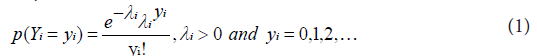
Consider we have n independent random variables denoted by Y1, Y2, …, Yn. Where yi denote neonatal death for ith mother in her life time. Poisson regression regression model for count data assumes that each observed count yi is drawn from a Poisson distribution with rate of occurrence of an event, parameter λi i=1, 2, …, n. Let Xi denote a vector of covariates in the study for the ith mother.
Then the Poisson equation of the model with rate parameter λi is given by:
The mean of the response variable λi is related with the linear predictor through the so called link function [9].
Now let X be nϰ (k+1) matrix of explanatory variables. The relationship between Yi and ith row vector of X, Xi, linked by g(λi), is the canonical link function given by:

where, Xi=(ϰi0, ϰi1, …, ϰik) is the ith row of covariate matrix, (with ϰi0=1indicating a vector of unity that represent the values for intercept term) and β= (β0, β1, …, βk) is unknown (k+1) dimensional vector of regression parameters.
The above two equations are called Poisson regression model or log-linear model.
Negative binomial regression model (NBR)
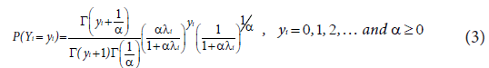
The main problem in the use of standard Poisson regression model, where there a more dispersed observations or if the data have excess zeros, another way of modeling such over-dispersed count data is a negative binomial (NB) distribution which can arise as a gamma mixture of Poisson distributions.
Let Y1, Y2, ..., Yn be a set of n independent random variables one parameterization of its probability density function is, then the negative binomial model given as:
Covariates can be introduced into a regression model based on the NB distribution via the relationship:
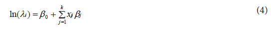
where xij is the ith observation corresponding to the jth covariate, k is the number of covariates in the model and βj is the jth regression parameter [10,11].
Zero-inflated regression models
One characteristic of the Poisson distribution is that the mean of the distribution is equal to the variance; however when there are excess zeros, probability of zero in the standard model will be less than the expected. The problem of standard models in underpredicting zeros and overpredicting ones is very common and sometimes this problem can be very severe when there are a lot of zeros in the distribution. In such cases, Zero inflated Poisson (ZIP) and Zero inflated negative binomial (ZINB) models can be used to account for excess zeros. The zero values in the ZIP model can be viewed as comprising two parts. One portion of the zero counts arises from the inflated part of the distribution and the other portion comes from what would be expected given a Poisson distribution with parameter λ [12].
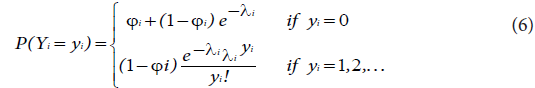
Zero-inflated Poisson regression model (ZIP): Generally, the zero-inflated probability mass function has the form:
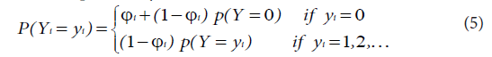
If Yi are independent random variables having a zero-inflated Poisson distribution, the zeros are assumed to arise in two ways corresponding to distinct underlying states. The first state occurs with probability Фi and produces only zeros, while the other state occurs with probability (1-Фi) and leads to a standard Poisson count with mean λi. In general, the zeros from the first state are called structural zeros and those from the Poisson distribution are called sampling zeros. This twostate process gives a simple two-component mixture distribution with probability mass function:
This is denoted by Yi ~ZIP (λi ,Фi ) such that 0 ≤ Фi <1, where λi is the mean of the non-zero outcomes that can be modelled with the associated explanatory covariates using a natural logarithmic link function as:

where Xi=(1, xi1, xi2, …, xik) is a (k+1) x1 vector of explanatory variable of the ith subject and β is (k+1)x1 vector of regression coefficient parameters. Фi (0 < Фi<1) is the probability of an excess zero (being in the zero mortality state) determined by a logit model. To predict membership in the “Always Zero” group, we can use the same variables or we can use a smaller subset of the variables or even different variables altogether, that is:

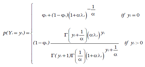
Zero-inflated negative binomial regression model (ZINB): The main difference between ZIP and ZINB model is that the Poisson distribution for the count data is replaced by the negative binomial distribution. The probability density function of a zero-inflated negative binomial distribution is a simple modification of the ZIP and is given by:
 (9)
(9)
where λi is the mean of the non-zero response that can be modelled with the associated explanatory covariates using a natural logarithm link function as defined in equation (7) and Фi is the probability of excess zeros which can be estimated by the logistic regression as defined in equation (8) [12].
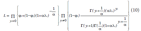
The ZINB model is a special case of a two-class finite mixture model like the ZIP model with mean E(Yi)=λi (1-Фi) and variance Var (Yi)=λi (1-Фi) (1+αλi+Фiλi), where the parameters λi and Фi depend on the covariates and α ≥ 0 is a scalar. Thus we have over-dispersion whenever either Фi or α is greater than 0. Thus, the equation in (10) reduces to NB when Фi=0 and to the ZIP when α=0.
The likelihood function for ZINB model is:
Assessing model fit
Overall regression test: Often after fitting a model it is good to assess how model is good fit. The null and alternative hypothesis for overall model goodness of fit may be symbolically stated as:
H0: β1=β2=β3=• • •=βK=0 versus Ha: Not all βj=0 for j=1, 2, 3, …, k
This can be tested using the deviance test with k degrees of freedom. The deviance (log likelihood ratio statistic) is given by Long [13]:
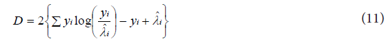
We reject the null hypothesis of no model goodness of fit for large value of the test for a given level of significance.
Test for significance of a single variable: The null hypothesis for this test may be stated as “Factor Xi does not have any value added to the prediction of the response given that other factors are already included in the model.”

To test such a null hypothesis, one can use
Where  is the estimated regression coefficient and
 is the estimate of the standard error of . This test statistic has the t-distribution with n-k-1 degree of freedom.
Test for over dispersion parameter: The negative binomial regression model reduces to the Poisson regression model when the over dispersion parameter is not significantly different from zero. To assess the adequacy of the negative binomial model over the Poisson regression model, we can test the hypothesis:
H0: α=0 versus Ha: α>0.
This is a test of significance of the over dispersion parameter α α. The presence of the over dispersion parameter α in the NB regression model is justified when the null hypothesis H0: α=0 is rejected. In order to test the above hypothesis a score test statistic is proposed. The general score test statistic for testing H0 can be given by:
where  is the predicted value from the Poisson regression model. Under the null hypothesis that the data follow a Poisson model, the limiting distribution of the score statistic is chi-squared with one degree of freedom [14,15].
Goodness of-fit tests: In this section, several goodness-of-fit measures will be briefly discussed, including the, likelihood ratio test, Vuong statistic, Akaike Information Criteria (AIC) and Bayesian Information Criteria (BSC).
Likelihood ratio: The advantage of using the maximum likelihood method is that the likelihood ratio test may be employed to assess the adequacy of the negative binomial over the Poisson because negative binomial will reduce to the Poisson when the dispersion parameter, α, equals zero. In this study a likelihood ratio was used to compare the Poisson with the negative binomial and zero-inflated Poisson with zeroinflated negative binomial since Poisson is nested on negative binomial and zero-inflated Poisson is nested in zero-inflated negative binomial. However this will not be used to compare Poisson or negative binomial with the zero inflated Poisson and negative binomial as long as these models are not nested one on the other.
The likelihood ratio statistic is given by:

where  and
and  are the model’s log likelihood under the alternative and null hypothesis, respectively. T has a chi-square distribution with one degrees of freedom. This method is not appropriate for models which are not nested. In such situations, we will use another method such as the Akakie information criteria (AIC) and Bayesian information criteria (BIC).
Akakie information criteria (AIC)
AIC is the most common means of identifying the model which fits well by comparing two or more than two models. It tries to balance the goodness of fit against the complexity of the model. It is given by:

where  denotes the log likelihood of a model that is to be compared with the other models and k is the number of parameter in the model including the intercept. A good model is the one which has the minimum AIC value [16,17].
The BIC is defined as:

where  denotes the log likelihood of the model, n is the sample size and k is the number of parameters in the model including the intercept. For this measure, the smaller the BIC, the better the model is [18].
Vuong statistic
Vuong has introduced a test which is a well suited method to compare zero-inflated regression models to standard non nested model for counts data. Suppose f1(yi/xi) and f2(yi/xi) denote the probability density functions of zero-inflated model (ZIP or ZINB) and parent (traditional) model (PO or NB), respectively. We want to test the following hypotheses:
H0: Two distribution functions are equivalent
Ha: Two distribution functions are different
Now we define
Where  and
and  are predicted probabilities of the corresponding models, respectively. Let
  and
and  denote the mean and standard deviation of the measurements mi. Then the Vuong statistic is defined as:
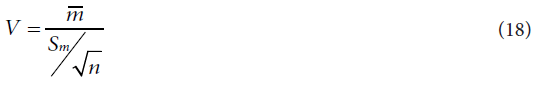
For large sample size and under the null hypothesis, the statistic V has an asymptotic standard normal distribution. Within the family of ZIP models, testing if a Poisson model is adequate corresponds to testing:
Where possible tests include the likelihood ratio test (LRT) and the score test. For a general ZIP regression model, the LRT for zeroinflation is given by:

Where are, respectively, the maximized loglikelihoods under the Poisson regression and the ZIP regression models [16,19].
Results
Table 2 below shows various descriptive statistics of neonatal deaths. The result shows that 76.8% of the mothers have not faced any neonatal death in their lifetime. If we observe the overall pattern of neonatal death at the national level, it is highly skewed to the right with excess zeroes (skewness=3.353, kurtosis=17.419) (Table 2).
| Number of neonatal death per woman | Number of mothers that experienced neonatal death | Percent | Cumulative Percent |
|---|---|---|---|
| 0 | 7069 | 76.8 | 76.8 |
| 1 | 1492 | 16.2 | 93.0 |
| 2 | 442 | 4.8 | 97.8 |
| 3 | 131 | 1.4 | 99.2 |
| 4+ | 75 | 0.8 | 100 |
| Total | 9209 | 100 | |
| Mean | 0.33326094 | ||
| Variance | 0.5751974 | ||
| Median | 0 | ||
| Skewness | 3.353 | ||
| Kurtosis | 17.419 |
Table 2: Number of mothers that experienced neonatal death.
Table 3 presents summary statistics of the variables that are assumed to affect neonatal mortality. The variables included are region, place of residence, mothers’ education level, husband/partner’s education level, number of antenatal visits, place of delivery, postnatal care, mothers’ occupation, religion, mothers age at first birth, source of water supply and availability of toilet facility (Table 3).
| Covariates | Category | Number of neonatal mortality per woman | ||||||
|---|---|---|---|---|---|---|---|---|
| 0 | 1 | 2 | 3 | 4+ | Neonatal death percent | Total | ||
| Region | 1 (Tigray) 2 (Affar) 3 (Amhara) 4 (Oromiya) 5 (Somali) 6 (Benishangul-Gumuz) 7 (SNN) 8 (Gambella) 9 (Harari) 10 (Addis Ababa) 11 (Dire Dawa) |
794 687 873 959 473 540 864 510 452 466 451 |
159 122 245 235 96 144 210 88 78 37 78 |
46 41 84 62 33 52 47 31 20 4 22 |
14 19 16 20 8 10 21 10 5 1 7 |
9 6 14 10 6 12 6 3 6 1 2 |
22.3 21.5 29.1 25.4 23.2 28.8 24.7 20.6 19.4 8.4 19.5 |
1022 (11.1%) 875 (9.5%) 1232 (13.4%) 1286 (14%) 616 (6.7%) 758 (8.2%) 1148 (12.5%) 642 (7%) 561 (6.1%) 509 (5.5%) 560 (6.1%) |
| Type of place of residence | 0 (Urban) 1 (Rural) |
1786 5283 |
234 1258 |
48 394 |
10 121 |
5 70 |
14.3 25.9 |
2083 (22.6%) 7126 (77.4%) |
| Mothers highest educational level | 1 (No education) 2 (Primary) 3 (Secondary and higher) |
4524 1960 585 |
1152 301 39 |
376 61 5 |
114 16 1 |
64 11 0 |
27.4 16.6 7.1 |
6230 (67.7%) 2349 (25.5%) 630 (6.8%) |
| Source of water supply | 1 (Pipe) 2 (Protected source) 3 (Unprotected source) |
2770 1419 2880 |
490 309 693 |
125 104 213 |
26 26 79 |
15 13 47 |
19.1 24.2 26.4 |
3426 (37.2%) 1871 (20.3%) 3912 (42.5%) |
| Availability of toilet facility | 0 (No facility) 1 (With facility) |
3214 3855 |
689 803 |
230 212 |
75 56 |
42 33 |
24.4 22.3 |
4250 (46.2%) 4959 (53.8%) |
| Religion | 1 (Orthodox) 2 (Protestant) 3 (Muslim) |
2702 1355 3012 |
553 277 662 |
161 76 205 |
36 31 64 |
27 12 36 |
22.3 22.6 24.3 |
3479 (37.8%) 1751 (19%) 3979 (43.2%) |
| Age of mothers at 1st birth | 0 (less than 20) 1 (20 and above) |
4277 2883 |
1074 418 |
323 119 |
93 38 |
60 15 |
26.6 14.8 |
5827 (63.3%) 3382 (36.7%) |
| Number of antenatal visits during pregnancy | 1 (No antenatal visits) 2 (1-3 visits) 3 (4 visits and above) |
4375 1316 1378 |
1070 240 182 |
335 67 40 |
106 15 10 |
66 4 5 |
26.5 19.9 14.7 |
5952 (64.6%) 1642 (17.8%) 1615 (17.5%) |
| Place of delivery | 0 (Home) 1 (health facility) |
4639 2430 |
960 532 |
267 175 |
80 51 |
41 34 |
22.5 24.6 |
5987 (65%) 3222 (35%) |
| postnatal care after delivery | 0 (No) 1 (Yes) |
4837 2232 |
956 536 |
259 183 |
78 53 |
41 34 |
21.6 26.5 |
6171 (67%) 3038 (33%) |
| Husband/partner's education level | 1 (No education) 2 (Primary) 3 (Secondary and higher) |
3453 2569 1074 |
886 498 108 |
294 126 22 |
91 34 6 |
59 15 1 |
27.8 20.8 9.3 |
4783 (51.9%) 3242 (35.2%) 1184 (12.9%) |
| Woman’s occupation | 1 (Not working) 2 (Agricultural sector) 3 (Nonagricultural sector) |
3551 1476 2042 |
708 389 395 |
215 118 109 |
71 32 28 |
33 22 20 |
22.4 27.5 21.3 |
4578 (49.7%) 2037 (22.1%) 2594 (28.2%) |
| Total | 7069 | 1492 | 442 | 131 | 75 | 23.2 | 9209 (100%) | |
Table 3: Summary statistics of some important socio-economic, demographic and environmental variables that are assumed to affect the neonatal death in Ethiopia.
The total number of women considered in this study was 9209 of which 2140 of them experienced neonatal death. Of the total number of neonatal deaths per woman, 14.3% and 25.9% of neonatal deaths have occurred in urban and rural areas, respectively. Another maternal variable that possibly has a strong bearing on the survival prospects of a child is the mother‘s age at the time of first birth. Regarding mothers’ age at first birth, 5827 (63.3%) of children were from mothers of age less than 20 years while the remaining 3382 (36.7%) were from mothers with age 20 years and above. Of these, 26.6% and 14.8% of children have died before the age of one month, respectively. Of the total of 9209 women included, 5987 (65%) have delivered at home and only 3038 (33%) have taken postnatal care. 26.5% of children from mothers who attended postnatal care have died before the age of one month. This figure is 21.6% for children whose mothers have not attended postnatal care.
Overall, more than three fourth 7126 (77.4%) of the respondents (mothers) live in rural areas, while less than one-fourth 2083 (22.6%) of them live in urban areas. From a theoretical perspective, place of residence is an important determinant of child survival. Mothers living in urban areas have a higher chance of getting health service and are aware of the benefit of medication than mothers who reside in rural areas. Table 3 reveals that the percentage of neonatal death for mothers who reside in rural and urban areas are about 26 and 14.3, respectively.
Table 3 also reveals that there is a decreasing trend in neonatal deaths with regards to education level of mothers (that is, neonatal deaths decrease as education level increases). In particular, the percentage of neonatal mortality was 27.4% for those with no education, 16.6% for those with primary education and 7.1% for those with secondary and higher education. Similarly fathers’ education shows higher mortality for neonates from illiterate fathers (27.8%) and is lower for fathers with secondary and higher education (9.3%).
If we consider the regional variation in neonatal death, Amhara and Benishangul-Gumuz had the highest proportion of neonatal death (29.1% and 28.8%, respectively), while Addis Ababa city administration has the lowest proportion of neonatal death (only 8.4%). As far as the numbers of antenatal visits are concerned, the neonatal death percentage decreased with an increase in the number of visits. Specifically, the neonatal death rate was 26.5% for woman who did not attend antenatal care, 19.9% for those who had between one and three visits and 14.7% for those who attended four or more visits (the minimum number recommended by WHO).
Results in Table 3 also show the summary statistics of sanitation indicators - source of water and type of toilet facility. Piped water supply reduces neonatal mortality directly by reducing the incidence of diarrhea that arises from the ingestion of contaminated water and food and indirectly when caregivers are able to devote more time to childcare instead of water collection activities. The results indicate that 3426 (37.2%) households had piped water while 3912 (42.5%) used water from unprotected source. Children to mothers with unprotected source of water supply accounted for 26.4% of neonatal death, while those to mothers with piped source of water supply accounted for 19% of neonatal deaths (Table 3).
Statistical data analysis and model comparison
The variable of interest in this study was the number of neonatal deaths per woman through her life time. Such data can be well fitted by the count data models rather than the linear regression model. Likelihood ratio test (LR), Akaike information criterion (AIC) and Bayesian information criterion (BIC) were used to compare the candidate models to identify the most appropriate model.
Development of count data regression models for determinants of neonatal mortality: Model identification
An initial step in the model building process is to identify sets of explanatory variables that have the potential for being included in the linear component of a multivariable count data regression model. We start with fitting univariable Poisson regression model. Based on univariate Poisson model we can identify candidate covariates to be considered for the multivariable model. Inclusion of such covariates will be based on a significant reduction in the value of -2Log L , where the bigger the reduction of this value, the better the fit. Including highest educational level of women, husband/partner’s educational attainment, number of antenatal visits, postnatal care, place of residence, region, place of delivery, age of mothers at first birth, religion, source of water supply, availability of toilet facility and occupation of mothers in the model, one at a time, result in a significant reduction in -2Log L using the chi-square test. Hence all these covariates are considered in the multivariable count data regression models.
Initially, we fitted Poisson model to identify the risk factors of neonatal mortality. The fitted Poisson model is then tested for overdispersion. However, the overdispersion might be due variation among observations or to excess zeroes. This brings the negative binomial model and the zero-inflated models into the picture. Thus, in order to select an appropriate model which fits the data well, four different models were considered, namely: the standard Poisson, negative binomial, zero-inflated Poisson and zero-inflated negative binomial models.
We start here first by checking the overall goodness of fit using deviance (likelihood ratio) statistic. Accordingly, the deviance-based chi-square test provided a chi-square value of 776.51 (p<0.0001) which would imply good fit for the model the fitted Poisson model. The following table display SAS and STATA output of the Poisson, negative binomial, zero-inflated Poisson and zero-inflated negative binomial regression models fit statistics (Table 4).
The score test statistic for over dispersion is χ2=1322.77 with p-value<0.0001, indicating that there is over-dispersion and the Poisson model is inappropriate. This is also supported by the Pearson Chisquare value divided by the degrees of freedom is close to one compared to the Poisson regression model, which one possible indication that there is over-dispersion.
| PRM | BIC=13955.15 χ2=12882.343 Df=981 |
AIC=13755.56 χ2/df=1.403 |
Prefer | Over | Evidence |
| Vs NBRM | BIC=13496.28 AIC=13289.57 χ2 =12882.343 Df=981 LR χ2=655.11 Sc. test=1322.77 |
diff.=458.87 diff.=465.99 χ2/df =1.0150 p-value<0.001 p-value<0.001 |
NBRM NBRM NBRM |
PRM PRM PRM |
Very strong P<0.001 |
| Vs ZIP | BIC=13701.6007 AIC=13302.4363 vuong=9.17 |
diff.=253.5493 diff.=453.1237 p-value<0.001 |
ZIP ZIP ZIP |
PRM PRM PRM |
Very strong P<0.001 |
| Vs ZINB | BIC=13458 AIC=13266 |
diff.=497.15 diff.=489.56 |
ZINB ZINB |
PRM PRM |
Very strong |
| NBRM | BIC=13496.28 | AIC=13289.57 | Prefer | Over | Evidence |
| Vs ZIP | BIC=13701.6007 AIC=13302.4363 |
diff.=-205.3207 diff.=-12.8663 |
NBRM NBRM |
ZIP ZIP |
Very strong |
| Vs ZINB | BIC=13458 AIC=13266 Vuong=4.73 |
diff.=38.28 diff.=23.57 p-value<0.001 |
ZINB ZINB ZINB |
NBRM NBRM NBRM |
Very strong P<0.001 |
| ZIP | BIC=13701.6007 | AIC=13302.436 | Prefer | Over | Evidence |
| Vs ZINB | BIC=13458 AIC=13266 LR χ2=136.61 |
diff.=243.6007 diff.=36.4363 p-value<0.001 |
ZINB ZINB ZINB |
ZIP ZIP ZIP |
Very strong P<0.001 |
Table 4: Tests and fit statistics for model comparisons.
Next we fit a negative binomial regression model with the same explanatory variables. The likelihood ratio test was used to compare the fit of the standard Poisson with NB regression model. This statistic was found to be statistically significant, indicating that NB regression model is a better fit to the data than the standard Poisson regression model (χ2(1)=655.11, p-value<0.0001). Thus, the observed data are better explained by the negative binomial than the Poisson model. Further as one can be seen from Table 4, the NB regression model is a better fit than the Poisson model since it has the smallest AIC (13289.57) as well as BIC (13496.28) values.
Still the reason for over dispersion is unknown thus, we need to fit the zero inflated count models. After fitting zero inflated models, we test H0: α=0 versus Ha: α>0 and H0: Ф=0 versus Ha: Ф>0 to identify whether the over dispersion is due to the presence of excess zeros or high variability in the non-zero outcomes. If the null hypothesis testing the inflation parameter H0: Ф=0 is not rejected, then the negative binomial model is appropriate and the over dispersion problem is due to the presence of high variability in the non-zero outcomes. However, if both parameters are significantly different from zero, then the zero inflated negative binomial regression models is more appropriate to fit the data.
Our result indicates that the over dispersion parameter (α) in the ZINB regression model is significantly different from zero (χ2=136.61 with P-value<0.001) and the likelihood ratio chi-square test statistic for testing the inflation parameter is also significant (χ2=600.317, P-value<0.0001).
Hence there was a high variability in the non-zero outcomes and the data excess of zeros. Thus, it is be better to use models which take into account both the high variability due to non-zero outcomes and excess of zeros simultaneously. Figure 1 below plots of difference between the observed probability of each count and the prediction from each of the four models. This result shows that ZINB distribution has the ability to reproduce the zeroes in the population better than ZIP distribution, which means that the ZINB model gives a good prediction of the number of neonatal deaths.
The other measure used to identify the appropriate model in this paper is the Vuong’s test. The Vuong test compares the ZIP model to the standard Poisson model by testing the null hypothesis that both models are equally similar to the observed distribution. The resulting statistic was statistically significant (V=9.17, p-value<0.0001), demonstrating that the ZIP model more reflects the observed data than standard Poisson due to the presence of excess zeroes. Similarly, the Vuong test that was used to compare ZINB versus negative binomial yields a test statistic of V=4.73 with p-value<0.0001. Thus, the Zero-inflated negative binomial regression model more accurately fits the number of neonatal deaths data compared to the standard negative binomial model.
Finally goodness of fit test for the fitted zero-inflated negative binomial regression model was assessed using the Pearson chi-square statistic. Accordingly, the Pearson’s chi-square test provided a chi-square value of 14144.59 (p-value<0.0001) which would imply good fit for the neonatal mortality data. Therefore, zero-inflated negative binomial (ZINB) regression model was found to be the most appropriate model which fits the data better than the other possible candidate models. Thus, in the analyses discussed below, the ZINB model is used (Figure 1).

Figure 1: Plots of difference between the observed probability of each count and the prediction from each of the four models.
Results in Table 5 provide estimates of the effect of some selected characteristics of mothers on the mortality of their neonate. The first set of coefficients is from the equation predicting counts for “not always zero” group. These coefficients can be interpreted the same way as regular negative binomial coefficients. The factors region, place of residence, education level of mothers, source of water supply, religion, age of mother at time of first birth, antenatal care, postnatal care and education level of husband/partner are statistically significant predictors of this count outcome. Availability of toilet facility, place of delivery and occupation of mothers are not statistically significant (Table 5).
| Covariates | Β | SE | Z | Sig. | Exp (β) | 95% C.I. for Exp (β) | |
|---|---|---|---|---|---|---|---|
| Lower | Upper | ||||||
| REGION (Addis Ababa) Tigray Affar Amhara Oromiya Somali Benishangul-Gumuz SNN Gambella Harari Dire Dawa |
0.421972 0.255199 0.500625 0.476696 0.466431 0.621206 0.453113 0.554933 0.431022 0.405160 |
0.181799 0.185402 0.177572 0.175607 0.187623 0.180291 0.184230 0.195482 0.188525 0.187673 |
2.32 1.38 2.822.71 2.49 2.45 2.46 2.84 2.29 2.16 |
0.020 0.169 0.005 0.007 0.013 0.001 0.014 0.005 0.022 0.031 |
1.5250 1.2907 1.6498 1.6107 1.5943 1.8612 1.5732 1.7418 1.5388 1.4995 |
1.06785 0.897465 1.16484 1.14169 1.10373 1.30714 1.09640 1.18740 1.06345 1.03803 |
2.17775 1.85629 2.33651 2.27250 2.30289 2.65003 2.25736 2.55505 2.22671 2.16624 |
| RESIDENCE (Urban) Rural |
0.273618 | 0.094689 | 2.89 | 0.004 | 1.3147 | 1.09202 | 1.58282 |
| EDUMOTH (No educ.) Primary Secondary and higher |
-0.38121 -1.0146 |
0.070689 0.180223 |
-5.39 -5.63 |
<0.001 <0.001 |
0.68303 0.36256 |
0.594665 0.254668 |
0.784536 0.516164 |
| SWATER (Pipe) Protected Unprotected |
0.116840 0.208672 |
0.081250 0.072379 |
1.44 2.88 |
0.150 0.004 |
1.1239 1.2320 | 0.958480 1.06909 |
1.31796 1.41982 |
| TOILET (No facility) With facility |
-0.08331 | 0.063562 | -1.31 | 0.190 | 0.92007 | 0.812297 | 1.04213 |
| RELIGION (Orthodox) Protestant Muslim |
0.275364 0.203513 |
0.099850 0.076923 |
2.76 2.61 | 0.006 0.009 |
1.3170 1.2257 |
1.08292 1.05221 |
1.60170 1.42780 |
| AGEMOTH (less than 20) 20 and above |
-0.28676 | 0.077869 | -4.72 | <0.001 | 0.75069 | 0.666355 | 0.845696 |
| ANC (No ANC visits) 1-3 visits 4 visits and above |
-0.22346 -0.38713 |
0.085546 0.084462 |
-2.61 -4.58 |
0.009 <0.001 |
0.79975 0.67900 | 0.676294 0.575408 |
0.945737 0.801245 |
| PDELIV (Home) Health facility |
-0.11033 | 0.111473 | -0.99 | 0.322 | 0.89554 | 0.719779 | 1.11422 |
| PNC (No) Yes |
0.366108 | 0.106920 | 3.42 | 0.001 | 1.4421 | 1.16946 | 1.77832 |
| EDUHUSB (No educ.) Primary Secondary and higher |
-0.27480 -0.26999 |
0.062792 0.124573 |
-4.38 -2.17 |
<0.001 0.030 |
0.75972 0.76338 |
0.671747 0.598005 |
0.859217 0.974493 |
| OCUMOTH (not working) Agricultural Non-agricultural |
-0.01470 0.091946 |
0.072727 0.066633 |
-0.20 1.38 |
0.840 0.168 |
0.98541 1.0963 |
0.854497 0.962084 |
1.13638 1.24925 |
| Intercept | -1.4693 | 0.190754 | -7.70 | <0.001 | |||
| 1.01997 | 0.110934 | ||||||
Reference categories are in parentheses
Table 5: Parameter estimates of the ZINB Model: Count equation, factor change in expected count for those “Not Always 0” group.
Concerning the regional disparity in neonatal mortality, the results in table 5 show that children in Amhara (OR: 1.65, 95% CI: 1.165-2.337), Benishangul-Gumuz (OR: 1.86, 95% CI: 1.307-2.65), Somali (OR: 1.59, 95% CI: 1.104-2.303), Oromiya (OR: 1.611, 95% CI: 1.142-2.273), Gambella (OR: 1.742, 95% IC: 1.187-2.555), SNNP (OR: 1.573, 95% CI: 1.096-2.257), Harari (OR: 1.54, 95% CI: 1.063-2.227), Tigray (OR: 1.525, 95% CI: 1.068-2.178) regions and Dire Dawa city administration (OR: 1.50, 95% CI: 1.038-2.166) are at a higher risk of experiencing neonatal death than children in Addis Ababa. The study shows that there is no significant difference in the risk of neonatal death between Affar region and Addis Ababa city administration.
Children born to a mother with secondary or higher schooling was associated with a 64% decreased risk of neonatal death compared to being born to mothers with no education, while primary education of the mothers decreases the risk of neonatal mortality by 32%, keeping all other covariates constant. Results in Table 5 indicate that children born from mothers whose age at first birth is greater than or equal to 20 have a significantly lower risk of mortality compared to those born from mothers whose age at first birth is less than 20. The risk of neonatal death was about 25% lower for births to mothers aged 20 and above compared with births to mothers less than age of 20 years (OR: 0.751, CI: 0.666- 0.846). This finding is consistent [20-22]. Children living in the rural areas had an increased risk to death compared to those children living in the urban areas. The risk of neonatal death was about 1.3147 times higher for a child whose mother resides in rural areas compared to their urban counterparts (OR: 1.315, 95% CI: 1.092-1.583). Theoretically, all things being equal, living in urban areas should be associated with a higher standard of living, better sanitation and better health facilities, among other things (Table 5).
The risk of neonatal mortality for those children whose mothers use unprotected source of water is 23% higher compared to those who use piped water supply (OR: 1.232, 95% CI: 1.069-1.420). There is no significant difference in neonatal mortality among those using piped water and protected source of water supply.
Further Table 3 shows that children of mothers whose husband has primary education and secondary and higher education have a significantly lower neonatal mortality risk than children of mothers whose husband has no education. Neonates born from mothers attending 1-3 antenatal care visits have a 20 percent lower risk of mortality than neonates born from mothers attending no antenatal care visits. Moreover, mothers with four or above antenatal care visits have a 32% lower risk than mothers with no antenatal care visits.
The second set of coefficients on the bottom half of table 5 predict the dichotomous outcome of group membership (i.e., “not always zero” versus “always zero” groups). The results show that women who delivered at health facility are less likely than those delivered at home to be in the “always zero” group. The odds for health facility delivery to be in the always zero group are 92% lower than for delivery at home. The odds for mothers with access to toilet facility to have no NM (being in always zero group) are 61% lower than those without availability of toilet facility. The results also indicate that the chance for membership in the “always zero” group (no neonatal death) increases by a factor of 3.67 for mothers whose religion is protestant holding all other variables constant (Table 5).
Discussion
The study has empirically investigated and identified the factors that are associated with the risk of neonatal mortality in Ethiopia based on EDHS 2016 data using four count regression methods. The study use retrospective study design. The main limitation of this study is it was difficult to gather all necessary variables and some variables did not get in a way we need. This may affect the association of outcome variable and the determinant factors. The confounding effect of unmeasured variables cannot be controlled. Some determinant factors like mode of delivery, birth weight and maternal smoking habits are a factors associate to neonatal mortality. But even if they are important determinant factors, we fail to include them in the analysis due to incompleteness of the data. Thus, any reader of this manuscript should take in to account the above limitations.
The findings of the study show that being born to a mother with education schooling was associated with decreased risk of neonatal death compared to being born to mothers with no education. Thus, educational level of mothers is an important and significant factor of neonatal mortality risks in Ethiopia. In literature most of the studies also report a negative relationship between neonatal death and mothers’ education level. They indicated that education improves the ability of mothers to implement simple health knowledge and facilitates their capacity to manipulate their environment including health care facilities, interact more effectively with health professionals, comply with treatment recommendations and keep their environment clean. Furthermore, educated women have greater control over health choices for their children [23-25].
Results also shows that children born from mothers whose age at first birth is greater than or equal to 20 have a significantly lower risk of mortality compared to those born from mothers whose age at first birth is less than 20. Children living in the rural areas had an increased risk to death compared to those children living in the urban areas. Theoretically, all things being equal, living in urban areas should be associated with a higher standard of living, better sanitation and better health facilities, among other things. Place of residence was found to have an association with neonatal mortality, such that children living in the rural areas had an increased risk to death compared to those children living in the urban areas. The risk of perinatal death was less for a child whose mother resides in urban areas compared to their rural counterparts. Theoretically, all things being equal, living in urban areas should be associated with a higher standard of living, better sanitation and better health facilities, among other things. This finding is in agreement with studies by which shows a significant association between place of residence, age at first birth and neonatal death [20-22,26].
Lack of clean water supply combined with little or no health care knowledge can provide routes for infections. The findings of this study show that mothers who use water from unprotected sources are at a higher risk of experiencing neonatal death than those who use pipe water. There is no significant difference in neonatal mortality among those using piped water and protected source of water supply.
Finally, husband education was found to be a significant predictor of neonatal mortality. Further result shows that children of mothers whose husband has primary education and secondary and higher education have a significantly lower neonatal mortality risk than children of mothers whose husband has no education. This finding is consistent with [24,27]. As an indicator of health care service utilization during pregnancy, antenatal care service factors demonstrated a significant association with neonatal mortality.
Conclusion
The study has empirically investigated and identified the factors that are associated with the risk of neonatal mortality in Ethiopia based on Ethiopian DHS 2011 data using methods of count data analysis [5]. Descriptive statistics and multivariable analyses were done to achieve this. In this study, after fitting four different count models it was found that NB, ZINB, regression models were better fitted the data than Poisson and ZIP. Furthermore the zero-inflated negative binomial model was better fitted with data which is characterized by excess zeros and high variability in the non-zero outcome.
According to the results of multivariable ZINB regression model it is found that the variables age of the mother at the time of the first birth, highest educational level the mother attained, number of antenatal visits during pregnancy, husband/partner’s educational attainment, postnatal care/seeking care after birth, place of residence, region, source of water supply and religion are the significant determinants of neonatal mortality in Ethiopia. However, place of delivery, access to toilet facility and mothers’ occupations were found to be insignificant factors of neonatal morality in Ethiopia.
In recent decades, Ethiopia has achieved significant declines in under-five and infant mortality rates. However, neonatal mortality rates have stayed higher than post-neonatal rates. Further interventions have to be done to reduce mortality rates among neonates. The findings presented in this study have the following research and policy implications:
• The survival experience of children in rural areas is much lower than those in urban areas. Thus, there is a need to increase access to maternal and child health services in rural areas.
• Improving the level of education of mothers is vital. Education of mothers plays an important role in survival of neonate and thus, health programs need to focus on supporting women with little or no education.
• Encourage, advocate and promote utilization of antenatal care services and the importance of following for both the mother and the newborn.
• The study revealed that children of households who use unprotected water as a source of drinking are at a higher risk of neonatal death. Thus, efforts should be made to improve access to safe/pipe drinking water and effective programs to reduce early childbearing of women should be implemented so as to decrease neonatal mortality.
Acknowledgement
We wish to acknowledge Macro International, USA for allowing us access to the 2011 Ethiopian Demographic and Health Survey dataset.
References
- WHO (2011) Guidelines on optimal feeding of low birth weight infants in low and middle income countries.
- Rajaratnam JK, Marcus JR, Flaxman AD, Wang H, Levin-Rector A, et al. (2010) Neonatal, post-neonatal, childhood and under-5 mortality for 187 countries, 1970-2010: A systematic analysis of progress towards Millennium Development Goal 4. Lancet 375: 1988-2008.
- CSA, ORC Macro (2005) EDHS. Addis Ababa, Ethiopia and Calverton, Maryland, USA.
- Oestergaard MZ, Inoue M, Yoshida S, Mahanani WR, Gore FM, et al. (2011) Neonatal mortality levels for 193 countries in 2009 with trends since 1990: A systematic analysis of progress, projections and priorities. PLoS Med.
- Morrow AL, Dawodu A (2004) Influencing birth outcomes in Nepal. Lancet 364: 914-915.
- Karlaftis MG, Tarko AP (1998) Heterogeneity considerations in accident modeling. Accid Anal Prev 30: 425-433.
- Mccullagh P, Nelder JA (1989) Generalized linear models, monographs on statistics and applied probability. 2nd edition, Chapman and Hall, London, UK.
- Lambert D (1992) Zero-inflated Poisson regression, with an application to defects in manufacturing. Technometrics 34: 1-14.
- Nelder JA, Wedderburn RWM (1972) Generalized linear models. J R Stat Soc 135: 370-384.
- Lawless JF (1987) Negative binomial and mixed Poisson regression. Can J Stat 15: 209-225.
- Cameron AC, Trivedi PK (1998) Regression analysis of count data. Cambridge University Press, UK.
- Natalia S, Gerstel N (2004) Explaining the gender gap in help to parents: The importance of employment. J Marriage Fam 66: 431-451.
- Long JS (1997) Regression models for categorical and limited dependent variables. Thousand Oaks, CA: Sage.
- Dean C, Lawless J F (1989) Tests for detecting over dispersion in poisson regression models. J Am Stat Assoc 84: 467-472.
- Yau Z (2006) Score tests for generalization and zore-inflation in count data modeling. Unpublished Ph.D Dissertation, University of South Caroline, Columbia.
- Agresti A (2002) Categorical data analysis. Wiley Interscience, New York.
- Akaike H (1973) Information theory and extension of the maximum likelihood principle. In: Petrov BN, Csaki F (Eds), Second international symposium on information theory, Akademiai Kiado, Budapest, pp: 267-281.
- Schwarz G (1978) Estimating the dimension of a model. Ann Stat 6: 461-464.
- Vuong QH (1989) Likelihood ratio tests for model selection and non-nested hypotheses. Econometrica 57: 307-333.
- Oji OS (2008) Risk factors for perinatal mortality in Nigeria: The role of place of delivery and delivery assistant.
- Hidalgo LA, Chedraui PA, Chevaz MJ (2005) Obstetrical and neonatal outcome in young adolescents of low socio-economic status: A case control study. Arch Gynecol Obstet 271: 207-211.
- Rutstein SO (2000) Factors associated with trends in infant and child mortality in developing countries during the 1990s. Bull World Health Organ 78: 1256-1270.
- Chernichovsky D, Meesook OA (1986) Utilization of health services in Indonesia. J Soc Sci Med 23: 611-620.
- Gabrysch S, Campbell OM (2009) Still too far to walk: Literature review of the determinants of delivery service use. BMC Pregnancy Childbirth 9: 34.
- Van-Ginneken J, Lob-Levyt J, Gove S (1996) Potential interventions for preventing pneumonia among young children in developing countries: Promoting maternal education. Trop Med Int Health 1: 283-294.
- Stanton, B, Langsten R (2000) Morbidity and mortality among Egyptian neonates and infants: Rates and associated factors. Ann Trop Med Parasitol 94: 817-829.
- Mats M (2010) Who can save the unseen? Studies on neonatal mortality in Quang Nihn province, Vietnam. Ph.D. dissertation, Uppsala University.
Citation: Woldeamanuel BT (2018) Statistical Analysis of Neonatal Mortality: A Case Study of Ethiopia. J Preg Child Health 5: 373. DOI: 10.4172/2376-127X.1000373
Copyright: ©2018 Woldeamanuel BT. This is an open-access article distributed under the terms of the Creative Commons Attribution License, which permits unrestricted use, distribution, and reproduction in any medium, provided the original author and source are credited
Share This Article
Recommended Journals
Open Access Journals
Article Tools
Article Usage
- Total views: 6259
- [From(publication date): 0-2018 - Dec 21, 2024]
- Breakdown by view type
- HTML page views: 4914
- PDF downloads: 1345