Research Article Open Access
Predicting Changes of Rainfall Erosivity and Hillslope Erosion across New South Wales, Australia
| Xihua Yang1*, Bofu Yu2, Qinggaozi Zhu3and De Li Liu4 | |
| 1New South Wales Office of Environment and Heritage, PO Box 644, Parramatta, NSW 2124, Australia | |
| 2Griffith School of Engineering, Nathan & Gold Coast Campuses, Griffith University, Australia | |
| 3School of Life Sciences, Faculty of Science, University of Technology, Sydney, Australia | |
| 4New South Wales Department of Primary Industries, Wagga Wagga Agricultural Institute, Wagga Wagga, NSW 2650, Australia | |
| *Corresponding Author : | Yang X New South Wales Office of Environment and Heritage Parramatta, NSW 2124, Australia Tel no: +61 2 98956517 Fax no: +61 2 98956548 E-mail: xihua.yang@environment.nsw.gov.au |
| Received February 22, 2015; Accepted March 18, 2016; Published March 22, 2016 | |
| Citation:Yang X, Yu B, Zhu Q, Liu DL (2016) Predicting Changes of Rainfall Erosivity and Hillslope Erosion across New South Wales, Australia. J Earth Sci Clim Change. 7:340. doi:10.4172/2157-7617.1000340 | |
| Copyright: © 2016 Yang X, et al. This is an open-access article distributed under the terms of the Creative Commons Attribution License, which permits unrestricted use, distribution, and reproduction in any medium, provided the original author and source are credited. | |
Visit for more related articles at Journal of Earth Science & Climatic Change
Abstract
New South Wales and Australia Capital Territory Regional Climate Modelling (NARCliM) project has produced a suite of 12 regional climate projections for south-east Australia spanning the range of likely future changes in climate. The aim of this study was to model and predict the impacts of climate change on rainfall erosivity and hillslope erosion risk across New South Wales using the NARCliM projections to assist the long-term climate change adaptation and regional planning. We developed a daily rainfall erosivity model for Southeast Australia to calculate monthly and annual rainfall erosivity values from the projected daily rainfall data for the baseline (1990-2009) and future periods (2020-2039 and 2060-2079). We produced monthly and annual hillslope erosion maps for these three periods using the Revised Universal Soil Loss Equation (RUSLE) with spatial interpolation to finer scale (100 m). Automated scripts have been developed in a geographic information system (GIS) to calculate the time-series rainfall erosivity and hillslope erosion so that the processes of large quantity climate projections are realistic, repeatable and portable. The model performance was assessed by comparing with data from Bureau of Meteorology for the baseline period and the overall coefficient of efficiency reached 0.9753 (RMSE 13.2%). Both rainfall erosivity and hillslope erosion risk are predicted to increase about 7% in the near future, and about 19% increase in the far future compared with the baseline period. The change is highly uneven in space and time, with the highest increase occurring in the Far-west in autumn. The rainfall erosivity is generally higher in summer and lower in winter, with about 10 times difference between February (highest) and July (lowest).
| Keywords |
| Rainfall erosivity; Hillslope erosion; Climate change; Impact assessment |
| Introduction |
| There are considerable seasonal and inter-annual changes in rainfall amount and intensity in many parts of the world. Climates in New South Wales (NSW) are highly variable; ranging from subtropical in the north-east part with summer-dominated rainfall to temperate climates with uniform or moderately winter rainfall in the southern part. The temporal and spatial variations in rainfall have enormous implications for soil conservation; food security; and natural resource management. One of the key climate drivers for soil erosion and land degradation is rainfall erosivity or R-factor; as defined in the Revised Universal Soil Loss Equation [1]. |
| Rainfall erosivity is largely a function of rainfall amount and peak rainfall intensity; and the R-factor; in units of MJ.mm.ha-1.hr-1.year-1; is a multi-annual average index that measures rainfall's kinetic energy and intensity to describe the effect of rainfall on sheet and rill erosion [1]. Among the factors used within RUSLE and its earlier version; the Universal Soil Loss Equation (USLE); rainfall erosivity is of high importance as precipitation is the driving force of erosion and has a direct impact on the detachment of soil particles; the breakdown of aggregates and the transport of eroded particles via runoff. A precise assessment of rainfall erosivity requires recordings of precipitation at short time intervals (1-60 minutes) for a period of at least several years. The rainfall erosivity is calculated by multiplying the kinetic energy by the maximum rainfall intensity during a period of 30 minutes for each rainstorm. The R-factor accumulates the rainfall erosivity of individual rainstorm events and averages this value over multiple years. When factors other than rainfall are held constant; soil losses due to water erosion are directly proportional to the level of rainfall erosivity [2]. When using the RUSLE; the R-factor is multiplied with other component factors relating to slope and slope-length (LS-factor); soil erodibility (K-factor); groundcover (C-factor) and soil conservation practices (P-factor) to predict the average annual soil loss per unit area. |
| Hillslope erosion is the major form of water erosion including sheet and rill erosion; and it has been identified as a significant emerging threat in NSW. The erosion information (hazard or risk; in units of t.ha-1.year-1) is required for informed target setting to protect and conserve land and biodiversity. In NSW; hillslope erosion risk (or the likelihood of) maps are routinely used in land-use planning; water quality monitoring; catchment management and forestry planting and harvesting operations. For example; hillslope erosion risk maps have been used to help assess the relative degree of constraints for various land-use purposes [3] and streamlined environmental assessment for bush fire hazard reduction work [4]. |
| Earlier work on rainfall erosivity in NSW was focused on the R-factor values calculated using pluviograph data at selected sites; and empirical relationships between the R-factor and rainfall intensity were used to map rainfall erosivity [5,6]. Isoerodent rainfall erosivity maps for NSW so produced are static in nature; and unable to capture the seasonal and inter-annual variability in rainfall erosivity. |
| While changes in rainfall amount and intensity are expected to have significant effects on rainfall erosivity and hillslope erosion; the magnitude of the impact is not well quantified because of the nonlinear nature of the relationship between rainfall amount and rainfall erosivity; and the extreme nature of large erosive events. Natural resource management targets can be more easily achieved if the hillslope erosion hazard and land degradation is well understood; and if the mean as well as extreme erosivity values are accurately mapped at a range of temporal and spatial scales. The high resolution R-factor maps; in both spatial and temporal contexts; can provide detailed information for climate (rainfall) impact assessment; and inform measurable and cost-effective means in sheet erosion identification and rehabilitation. |
| A daily erosivity model has been developed and the required parameter values can be estimated from long-term climate averages or geographical attributes to allow efficient large-scale erosion assessment [7-9]. The technology has been widely used to estimate the magnitude and spatial distribution of hillslope erosion at a range of temporal and spatial scales [9,10]; and for assessment of the impact of projected future climates on hillslope erosion and catchment health in NSW [11]. With the regional relationship for model parameters [8,9]; rainfall erosivity can now be estimated with gridded daily rainfall data anywhere in Australia. The improved rainfall erosivity model may also have the potential to predict spatial and temporal changes of rainfall erosivity and hillslope erosion risk using future climate projections. |
| New South Wales and Australia Capital Territory Regional Climate Modelling (NARCliM) funded by the NSW Office of Environment and Heritage (OEH) is an initiative to produce regional climate projections for South-East Australia [12]. Twelve climate member ensembles were used to provide robust and unbiased projections that span the range of likely future changes in climate. A wide variety of climate variables have been made available at high temporal and spatial resolution for use in impacts and adaptation research including precipitation at daily and hourly steps which are the major input data in this study. |
| The objectives of this study were to 1) predict future changes in rainfall erosivity and hillslope erosion by comparing with baseline period; 2) assess the impacts of climate (rainfall) change on rainfall erosivity and hillslope erosion based on the state planning regions (SPR); and 3) produce finer scale (up to 100 m) time-series R-factor and erosion maps at monthly and annual steps up to 2079 for future climate change adaptation. This paper outlines the data and methods used to produce the time series of R-factor maps for NSW and SEA; and the impact assessment of baseline and future rainfall on erosivity and hillslope erosion risk across NSW. |
| Data and methods |
| Study area and input datasets |
| The NARCliM model domain is bounded by 21.669º-39.749ºS and 132.724º-165.725ºE and it is the landmass area within the domain extent [12]. There are 124 rainfall pluviograph sites within SEA which can be used for model development; such as the geo-referenced model parameters [13] representing the regional relationships and spatial distribution. |
| The input datasets include: 1) NARCliM projected daily rainfall with bias correction for all 12 member ensembles from four Global Climate Models (GCMs) and three Regional Climate Models (RCMs) (Table 1) for three time slices: baseline (1990-2009); near future (2020-2039) and far future (2060-2079); 2) Gridded Daily Rainfall from Bureau of Meteorology [14] (BoM 2009) for historical periods (1910-2013; 1961- 1990; 1990-2009) as a reference or baseline; 3) 1-second (about 30 m) hydrologically corrected Digital Elevation Model (DEM-H;) [15]; and 4) NSW Great Soil Groups (GSG) map and Soil and Land Information System (SALIS). |
| For reporting purposes; the spatial variation and comparisons are focused on state planning regions (SPRs) of NSW. This is required by the NSW Regional Action Plans which focus on actions the NSW Government will take to improve outcomes in each region. In addition to SPRs; land use and bioregions are also used in the impact assessment and comparisons of changes in rainfall erosivity and hillslope erosion. |
| The daily rainfall erosivity model |
| The daily rainfall erosivity model follows that of Yu and Rosewell [7] and Lu and Yu [9] with significant improvements on model parameters [16]. Briefly; the model to estimate the sum of total kinetic energy from storms and the peak 30-min (5 x 6-min) intensity values for the month j (or monthly rainfall erosivity in units of MJ.mm.ha-1. hr-1.month-1) from daily rainfall amounts is based on |
| where Rd is the daily rainfall amount (mm/day); N is the number of rain days in the month; and α; β; η; and ω are model parameters. The model assumes a non-linear relationship between daily rainfall amount and daily rainfall erosivity values via the parameter β. For the same amount of rainfall; however; rainfall erosivity can vary depending on the time of year and the location; especially the latitude and elevation. The remaining three parameters in Equation (1); namely α; η; and ω; were used in an attempt to capture these effects in a relatively parsimonious fashion. |
| For the exponent β; the following regression equation was developed for SEA: |
| where L is the latitude in decimal degrees; which is a negative value for the southern hemisphere. Equation (2) was based on pluviograph calibrated parameter values [16] for the exponent β for these 124 sites as shown in Figure 1. This suggests that at the higher latitude; the relationship between rainfall amount and rainfall erosivity is much more non-linear. At the higher latitude; there is a much greater range of rainfall intensity than in the subtropical and tropical regions where the rainfall intensity is; in general; consistently high. |
| Once the exponent β is determined from equation (2); the reference α0 value can be determined from the following equation: |
| Note also that when Equation (3) is used to estimate the coefficient α0 from the exponent β; a correction factor of 1.05 needs to be applied to remove the bias introduced in anti-log transformations [17]. |
| Multi-variable regression relationship for the departures is given by: |
| where E is the elevation above the sea level in metres from DEM (DEM-H). Equation (4) was also based on calibrated parameter values from the 124 sites. The equation suggests that for the same amount of rain in the same month; the rainfall erosivity is likely to be higher at lower latitude (northward) and at lower elevation. As the latitude increases; i.e. moving from south to north in NSW (negative latitude); rainfall erosivity would increase for a given amount of rain. Likewise; as the elevation increases; rainfall would become less and rainfall erosivity would decrease for a given amount of rain as the regression suggests. This may well be related to the variation in the size distribution of rain drops as a function of the latitude and elevation. |
| The annual rainfall erosivity (R-factor; in units of MJ.mm.ha-1. hr-1.month-1) for a given year is simply the sum of the monthly rainfall erosivity in the year as calculated using Equation 1. |
| Hillslope erosion |
| The time-series (monthly) rainfall erosivity layers produced in this study are further used to estimate monthly hillslope erosion based on RUSLE [1]: |
| where A is the predicted hillslope erosion (t.ha-1.month-1); R is rainfall erosivity (R) factor (MJ.mm.ha-1.hr-1.month-1) as calculated above; K is the soil erodibility factor (t.ha.hr.ha-1MJ-1mm-1); LS is the slope and steepness factor (unitless). Note that the cover and management (C) factor (unitless) and erosion control (P) factor (unitless) in the future were not considered in this work as the relevant future data are not available; thus the results are the likelihood of hillslope erosion or erosion risk. The K-factor map was prepared from the GSG and LS-factor calculated from DEM-H [11]. The hillslope erosion was calculated monthly and annually from for each year. |
| Procedures |
| Due to the large quantity of input datasets from different sources (refer 2.1); automated GIS scripts have been developed to process the daily rainfall data and calculate the monthly and annual rainfall erosivity. The procedures include: |
| • convert the NARCliM modelled daily rainfall (in NetCDF) to ASCII and ESRI ArcInfo grids (total 262;980 data layers); |
| • check and remove abnormal rainfall values (e.g. >350 mm/ day); |
| • calculate daily and monthly Rd (the right-most section of Equation 1); |
| • interpolate monthly Rd to finer resolution (100 m) and fill nondata gaps originating from NARCliM rainfall projections; |
| • calculate monthly rainfall erosivity (Equation 1); |
| • calculate annual rainfall erosivity (sum of monthly rainfall erosivity); |
| • calculate monthly hillslope erosion using RUSLE (Equation 5); |
| • calculate annual hillslope erosion (sum of monthly soil loss); and |
| • calculate mean rainfall erosivity and hillslope erosion for all periods and all member ensembles; and their seasonal means. |
| Model performance assessment |
| Model performance is measured by the coefficient of efficiency; Ec [18] as: |
| |
| where yi and yˆi are observed and modelled values; respectively; y is the average of observed values; and M is the sample size. Essentially; c E is an indicator of how close the scatter of predicted versus actual values are to the 1:1 line which can be considered as a measure of model efficiency for any other types of models. In addition; mean relative error (MRE) and root mean squared error (RMSE) are also used for accuracy assessment. |
| The accuracy assessment compares the annual mean rainfall erosivity in the baseline period (1990-2009) from NARCliM projected daily rainfall (all 12 member ensembles) against that from the BoM gridded daily rainfall for the same period. The latter has been assessed against the calibrated rainfall erosivity in a recent study (Yang & Yu 2015). |
| Results and Discussion |
| GIS layers and accuracy assessment |
| Based on the daily rainfall erosivity model (Equations 1-4) and procedures as outlined above; we produced monthly and annual rainfall erosivity GIS layers for all of NSW and SEA from the daily rainfall data from all 12 NARCliM ensembles for all the three projection periods (1990-2009; 2020-2039; 2060-2079). Multi-model mean annual and seasonal rainfall erosivity and the changes were further calculated and spatially interpolated into fine spatial resolution (100 m) using a spatial interpolation method (Spline). |
| The modelled rainfall erosivity data were further used to estimate hillslope erosion based on RUSLE (Equation 5); and the same sets of hillslope erosion layers (monthly; seasonal and annual) have been produced for the same periods for NSW and SEA; as well as spatial interpolation and multi-model means. In total over 30;000 GIS layers were produced and the entire calculation took about three months on a high-end PC (Thinkstation D30 Workstation) with 3.7 GHz processor and 128 GB memory. |
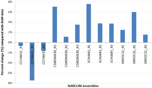
| Rainfall erosivity values calculated from the 12 NARCliM member ensembles vary significantly (Figure 1). Compared with the results from the gridded daily rainfall data (BoM 2009); the percent changes of mean rainfall erosivity values from the 12 member ensembles range from about -8% to about 8%; with an overall change of about 2% (2.26%). All 12 member ensembles; except GCM CCCMA3.1; resulted in an overestimate of the mean annual rainfall erosivity; while results from CCCMA31_R1 and CSIROMK30_R2 have less than 1% variation compared to the BoM mean value. CCCMA31_R3 and MIROC32_R3 have less than 2% variation compared to the result from BoM data. The overall 2.26% overestimate of rainfall erosivity is due to the 1.65% overall increase in the NARCliM projected mean annual rainfall (525 mm.year-1) compared with the BoM rainfall (519 mm.year-1) in the same period (1990-2009). |
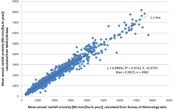
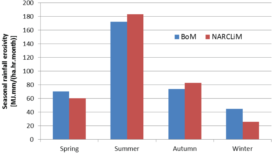
| Adequate random sampling points (4991 in total) were used to sample and assess the accuracy of the modelled rainfall erosivity from the NARCliM projections. The GIS modelled mean annual rainfall erosivity values using the NARCliM projected daily rainfall were compared with those calculated using the BoM gridded daily rainfall data at 5 km spatial resolution (BoM 2009) for the baseline period (1990-2009). The overall Ec (Eq. 6) for the rainfall erosivity is 0.9753 (R2 = 0.9762); overall bias is 0.9925 suggesting a slight under-estimation; and RMSE is 13.2% or 143 (MJ.mm.ha-1.hr-1. year-1) indicating the relative size of the error bars from the 1:1 line (Figure 2). The seasonal patterns between the NARCliM and BoM data are also similar; both showing high rainfall erosivity in summer and low in winter (Figure 3). |
| Baseline rainfall erosivity and hillslope erosion |
| Three historical baseline periods were used to describe and compare the overall trend and changes in rainfall erosivity and erosion risk. These include a 20-year baseline period (1990-2009) for comparison with the NARCliM projections of the same length; and a standard 30-year baseline period (1961-1990) and a longer (100+ years) baseline period (1910-2013) for better understanding the overall historic changes. The rainfall erosivity values for the three baseline periods were calculated using the achieved daily rainfall grids from BoM. |
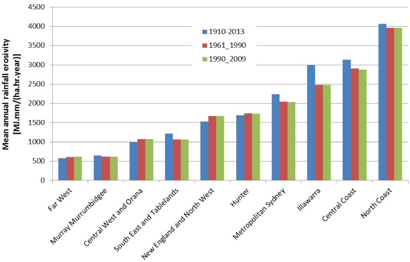
| There is great similarity in the seasonal changes in rainfall erosivity in all three baseline periods; revealing higher erosivity in summer and lower in winter; about seven times difference between July and February. The spatial patterns of rainfall erosivity in the three historical periods are also very similar and they all show the general trends of rainfall erosivity; increasing from west to east and south to north (Figure 4). The variation across NSW state planning regions ranges from the lowest in the Far West (about 500 MJ.mm.ha-1.hr-1.year-1) to the highest in the North Coast (about 4000 MJ.mm.ha-1.hr-1.year- 1). This suggests that erosion risk could vary about eight times across the SPRs. Such relatively large regional variations were also noted in previous studies in NSW [19]. |
| The comparison shows that the mean annual rainfall erosivity values among these baseline periods vary by up to 7%. These variations show that the same baseline period should be used throughout the comparisons and assessment process for current and future changes. Using different baseline periods could result in a variation of up to 7%. For this study; the NARCliM projection for the period 1990-2009 was used as the baseline to compare with the near (2020-2039) and far future (2060-2079) projections as they were from the same source (NARCliM) with the same time slice (20-year period). |
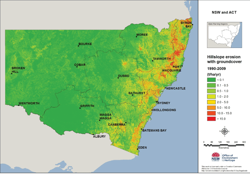
| Hillslope erosion in these baseline periods has similar seasonal and spatial variations as that of rainfall erosivity. Figure 5 shows the mean annual hillslope erosion (t.ha-1.year-1) for the baseline period (1990- 2009) with the current groundcover conditions. The map shows the high erosion risk areas are generally along the Great Dividing Range due to the combined effects of steep terrains and high rainfall erosivity. North Coast; Hunter and Central Coast regions are predicted to have a mean hillslope erosion rate over 4 t.ha-1.year-1 in the near and fur futures even if the current groundcover conditions are maintained. This is primarily due to the presence of more erosive rainfall (storm events) and steep terrains in these regions (Yang 2015). |
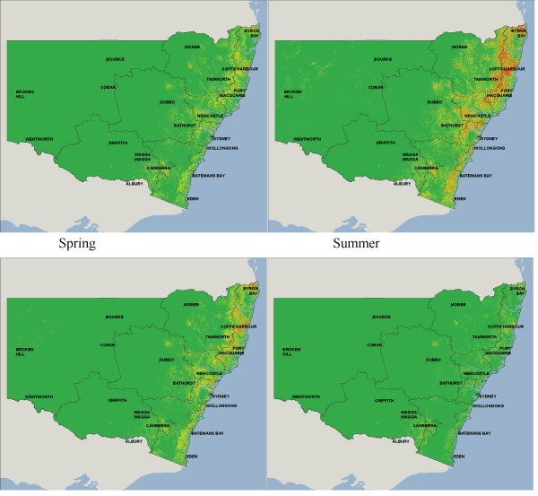
| Figure 6 shows the mean seasonal (monthly mean in a season) hillslope erosion (t.ha-1.season-1) for the baseline period (1990-2009) with the current groundcover conditions. It shows great seasonal variation (about a 7-fold difference) with the highest erosion rate in summer and the lowest in winter. |
| The high erosion risk areas (i.e. North Coast and Central Coast regions) in summer have implications for water quality; agricultural productivity and biodiversity due to the significance of the regions and their current erosion levels. It is important to maintain good groundcover in these areas; otherwise there will be a significant increase in erosion risk in these regions. |
| As these maps are in time series for a long period; they are useful for continuous and consistent soil condition monitoring and management. For example; a storm event in the severely burnt Warrumbungle National Park in February 2013; which lasted approximately 45 minutes; caused considerable flooding and hillslope erosion with the catastrophic consequence of long-term landscape change in this iconic park. The time-series erosion risk maps (i.e. at monthly steps) could be used to monitor post-fire erosion and recovery. |
| Future changes in rainfall erosivity and hillslope erosion |
| Geographic changes: Predicted future changes (%) in rainfall erosivity from the 12 NARCliM member ensembles vary significantly. To minimise the model biases; the mean annual rainfall erosivity values from all 12 member ensembles are used to assess the overall changes in rainfall erosivity in the near and far future periods (2020-2039; 2060- 2079). |
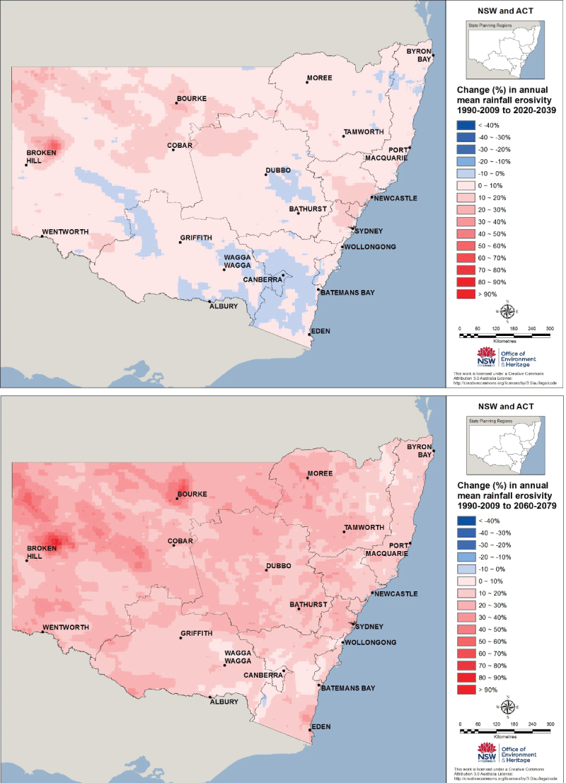
| Compared with the baseline period (1990-2009); the mean annual rainfall erosivity in NSW is predicted to increase in the future. Statewide; there is about a 7% increase in the near future (2020-2039) and about a 19% increase in the far future (2060-2079). Figure 7 shows the percent change in rainfall erosivity across NSW in the near and far futures. The mean annual rainfall erosivity and the future changes in each SPR in relation to the baseline period are summarised in Table 2. The changes vary from 1.4% (South East and Table lands) to 13.8% (Central Coast) in the near future; and from 13.9% (Illawarra) to 27.5% (Far West) in the far future. |
| Changes in rainfall erosivity lead to changes in hillslope erosion assuming other RUSLE factors remain unchanged. The corresponding changes in hillslope erosion in each SPR in relation to the baseline period are summarised in Table 3. It assumes that the baseline groundcover conditions are maintained in the future. |
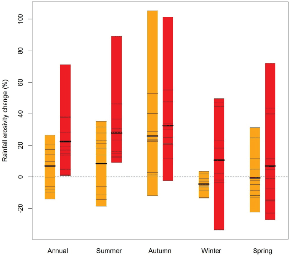
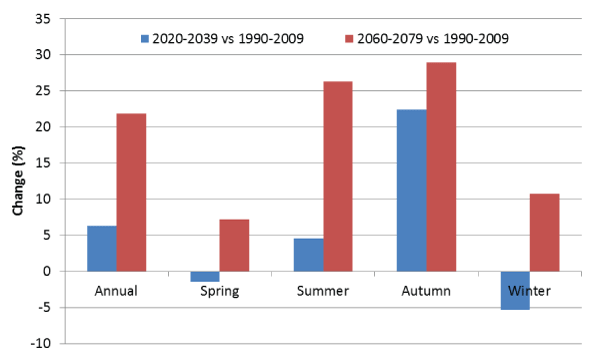
| Seasonal changes: The seasonal changes in rainfall erosivity are highly uneven and variable among the 12 member ensembles. Figure 8 shows future seasonal and annual changes (%) compared with the baseline period among the 12 member ensembles. The variations range from -22.2% in spring to 105.3% in autumn for the near future period; and from -33.7% in winter to 101.2% in autumn for the far future period. The majority of models agree that erosivity will increase in summer for both the near future (8/12) and the far future (12/12). For autumn the majority of models project an average increase across the state in the near future (11/12) and the far future (11/12). There is less clarity in the changes to winter and spring erosivity; due to the complex nature of the changes in rainfall in those seasons. |
| It is predicted that the rainfall erosivity will generally increase in all seasons across NSW. Autumn will have the highest increase with about 22% in the near future and about 29% in the far future. Rainfall erosivity in summer is also predicted to increase significantly; about 5% in the near future and 26% in far future. The only exception is the slight decrease in the near future in spring and winter (Figure 9). |
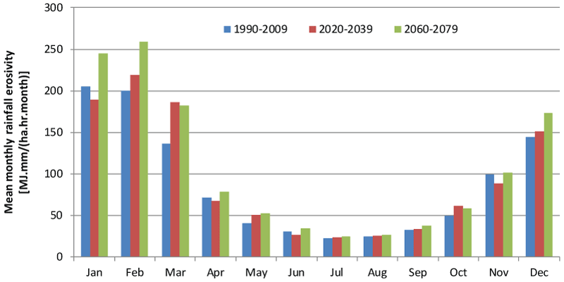
| One distinct advantage in using the daily erosivity model in GIS is the ability to predict monthly or seasonal rainfall erosivity and its distribution anywhere in NSW (Yang & Yu 2015). Figure 10 shows the modelled mean monthly rainfall erosivity in the three periods from the NARCliM projections. The seasonal variation is similar to the pattern of the baseline periods showing high rainfall erosivity in summer and low in winter; about a seven-fold difference between February and July. The seasonal distribution of rainfall erosivity will have significant impacts on hillslope erosion. This implies that when all other RUSLE factors remain unchanged; the seasonality of rainfall erosivity alone could cause an approximately seven-fold difference in soil loss. |
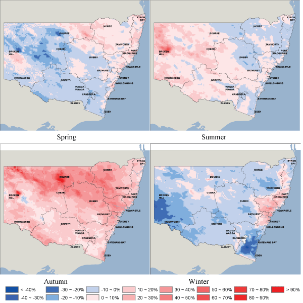
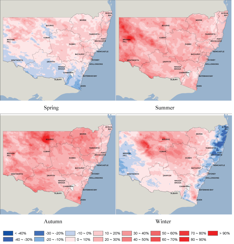
| Figures 11 and 12 show the seasonal changes in rainfall erosivity in the future; spatially across NSW. Rainfall erosivity generally increases in all seasons in most areas of the state in the future. However; Southern Coast in the near future and North Coast in the far future are predicted to decrease in rainfall erosivity in winter (about 20-30%). This is due to predicted decreases in rainfall in winter in these areas. Contrastingly; Broken Hill and Bourke are projected to have a significant increase in erosivity in the near and far futures (>70% change in autumn). Though the relative changes are high there is little impact on hillslope erosion as historically these areas do not experience significant water erosion (less than 0.1 t.ha-1year-1 due to relatively flat terrains. Even if the rainfall erosivity in these areas increases by 90% in the future; the actual hillslope erosion would be 0.19 t.ha-1year-1; which is still considered very low compared with the coastal areas. |
| Importantly; however; areas along the coast and the ranges are projected to experience up to a 40% increase in erosivity in the near and far futures; especially in summer and autumn. Erosivity is also projected to increase considerably in the Central Coast region in winter (20-30%). These increases have implications for water quality; agricultural productivity and biodiversity due to the significance of the regions and their current high erosion risk. It is important to maintain good groundcover in these areas; otherwise there will be a significant increase in erosion risk. |
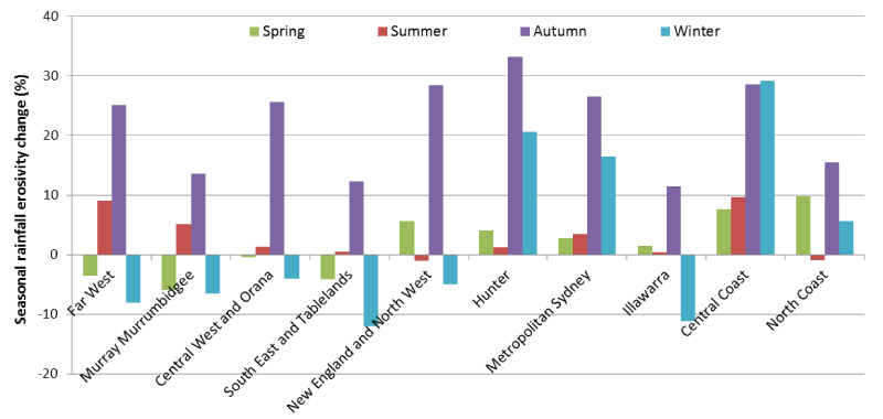
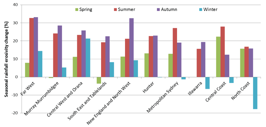
| The seasonal change is highly uneven across SPRs; ranging from -12% in South East and Tablelands (in winter) to 33% in Hunter (in autumn) in the near future (Figure 13). The far future shows more increases across all SPRs in general; particularly in western NSW; ranging from -18% in North Coast (in winter) to 33% in Far West (in autumn). In contrast; some coastal regions are predicted to experience decreases in rainfall erosivity in the next 50 years; such as North Coast; Central Coast and Illawarra in winter (Figure 14). |
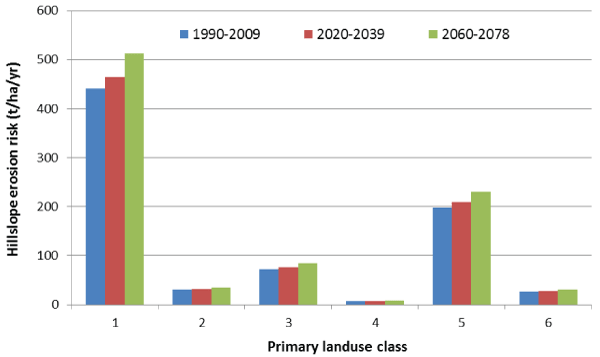
| Land use and hillslope erosion risk: Hillslope erosion has implications for different land uses. There are six primary landuse types in NSW based on Australian Land Use and Management Classification Version 7 [20] and they are: 1) Conservation and natural environments; 2) Production from relatively natural environments; 3) Production from dryland agriculture and plantations; 4) Production from irrigated agriculture and plantations; 5) Intensive uses; and 6) Water. The predicted hillslope erosion risk for each primary land use is shown on Figure 15. |
| The land-use type ‘Conservation and natural environments’ (Class 1) covers about 15% of NSW. Figure 15 shows this class has the highest erosion risk as it includes national parks and conservation areas which are normally in steep terrains with a high frequency of bushfires. However; the actual erosion in these areas can be reduced considerably if groundcover is maintained [21]. |
| The ‘Intensive uses’ category (Class 5) is projected to have the second highest erosion risk (Figure 15) due to the combined effects of groundcover (bare soil); terrain and rainfall erosivity. This category also includes urban areas and mining; the actual erosion risk is expected to be reduced if erosion control measures (such as concrete or brick surfaces) are in place. |
| The risk of hillslope erosion on NSW agricultural and plantation lands (Classes 3 and 4) is expected to slightly increase; largely due to the topographic factor of the land uses as they are normally in flat terrains. The ‘Intensive uses’ category (Class 5) will still have high erosion risk due to the combined effects of terrain and rainfall erosivity. This category includes urban areas; the actual erosion risk is expected to be far less than projected as most urban areas are paved (concrete or bricks) rather than bare soil as the model assumed. This detailed information could help decision-makers to better target and design the best management practices for a given land use type or region. |
| Conclusion and Further Studies |
| NARCliM projected daily rainfall data have been used to predicted rainfall erosivity and hillslope erosion risk and their future changes across NSW and SEA. Rainfall erosivity and hillslope erosion risk across NSW are predicted to increase by about 7% in the near future (2020- 2039); and by about 19% in the next 50 years. The change is highly uneven in space and in time; and the spatial and temporal patterns provide meaningful information for climate change assessment and adaptation. Rainfall erosivity and hillslope erosion are mostly greater in summer than in other seasons. This suggests that summer (particularly February) is the critical season for hillslope erosion prevention and management. The 7-19% extra hillslope erosion in the future for unprotected soil is a serious concern. Review of erosion and sediment control standards for construction and re-assessment of land management practices may be required for the predicted high risk areas. |
| The improved daily rainfall erosivity model performed well and the overall model efficiency (Ec) for estimated rainfall erosivity values is greater than 0.97; with an overall bias slightly greater than one. The set of regional relationships for the model parameters are highly recommended for use for NSW and SEA to estimate and map rainfall erosivity and its spatial and seasonal distribution. |
| The model outputs are available at high temporal and spatial resolution for use in climate impact assessment and hillslope erosion monitoring for the past; current and future. The time series of rainfall erosivity and hillslope erosion GIS layers in such high spatial (100 m) and temporal (monthly to annual) resolution across SEA are the first available in Australia. The baseline rainfall erosivity layers for the period of climate normals (1961-1990); a reference period (1990-2009) and a longer baseline period (1910-2013) have been produced for better climate change comparisons. |
| This study has demonstrated an appropriate approach for modelling and mapping monthly and annual rainfall erosivity from daily rainfall data for SEA which is also readily applicable to other regions. The methods have been successfully implemented in GIS for efficient calculation and mapping of the spatial and temporal variation of rainfall erosivity and hillslope erosion across SEA. With the automated GIS process developed in this study; the erosivity maps and erosion modelling can be readily upgraded when better rainfall data and models become available. The spatial interpolation greatly enhanced the level of detail; which is useful for assessing erosion hazard and determining the timing of erosion control practices. The time series of high resolution rainfall erosivity and hillslope erosion maps can provide detailed information for climate (rainfall) impact assessment; and a cost-effective means for hillslope erosion hazard identification and rehabilitation. |
| Further work will include examining and predicting the impacts of rainfall extremes on rainfall erosivity and hillslope erosion as soil erosion happens mostly during a few severe storm or extreme events. These will provide more useful information for storm impacts on bushfire affected areas so that one can optimise appropriate remedial activities for individual storm events. |
References
|
Tables and Figures at a glance
| Table 1 | Table 2 | Table 3 |
Figures at a glance
 |
 |
 |
 |
 |
| Figure 1 | Figure 2 | Figure 3 | Figure 4 | Figure 5 |
 |
 |
 |
 |
 |
| Figure 6 | Figure 7 | Figure 8 | Figure 9 | Figure 10 |
 |
 |
 |
 |
 |
| Figure 11 | Figure 12 | Figure 13 | Figure 14 | Figure 15 |
Relevant Topics
- Atmosphere
- Atmospheric Chemistry
- Atmospheric inversions
- Biosphere
- Chemical Oceanography
- Climate Modeling
- Crystallography
- Disaster Science
- Earth Science
- Ecology
- Environmental Degradation
- Gemology
- Geochemistry
- Geochronology
- Geomicrobiology
- Geomorphology
- Geosciences
- Geostatistics
- Glaciology
- Microplastic Pollution
- Mineralogy
- Soil Erosion and Land Degradation
Recommended Journals
Article Tools
Article Usage
- Total views: 11521
- [From(publication date):
March-2016 - Jul 03, 2025] - Breakdown by view type
- HTML page views : 10516
- PDF downloads : 1005
