Research Article Open Access
Optimization of CO2 Storage in Saline Aquifers using the Raven Software
Barham S Mahmood*
Institute of Petroleum Engineering, Heriot Watt University, Edinburgh Campus, Edinburgh EH14 4AS, UK
- *Corresponding Author:
- Barham S Mahmood
Institute of Petroleum Engineering
Heriot Watt University, Edinburgh Campus
Edinburgh EH14 4AS, UK
Tel: + 9647703605782
E-mail: barham.sabir@ koyauniversity.org
Received Date: August 03, 2015; Accepted Date: November 25, 2015; Published Date: December 01, 2015
Citation: Mahmood BS (2015) Optimization of CO2 Storage in Saline Aquifers using the Raven Software. J Ecosys Ecograph 5:172. doi:10.4172/2157-7625.1000172
Copyright: © 2015 Mahmood BS. This is an open-access article distributed under the terms of the Creative Commons Attribution License, which permits unrestricted use, distribution, and reproduction in any medium, provided the original author and source are credited.
Visit for more related articles at Journal of Ecosystem & Ecography
Abstract
CO2 storage in deep saline aquifer is still at its infancy and not yet matured for large scale industrial development due to the considerable uncertainties that still exist regarding storage capacity and safety. At the same time, because this is an expensive process, so engineers wish to store as much CO2 as possible within a particular saline formation. However, injecting huge amounts of CO2 into the particular saline formation pose significant technical issue such as pressure build-up and CO2 leakage. Therefore, in order to fully exploit it is potential, optimum injection strategies need to be investigated. In this paper we examine a realistic model of deep saline aquifer and conduct optimization study on some simulation parameters by applying multi-objective particle swarm optimization algorithm (MOPSO) to Enhance CO2 storage capacity and safety by, 1) Maximize total injected CO2, 2) Minimize pressure build-up in the center of the field and 3) Minimize CO2 leakage at the edges of the aquifer. The result of this study shows that when changing the number of wells from 5 to 7 injectors the possible storage capacity for dome A is increased by 4%. However, the maximum CO2 leakage did not reach the criterion of 0.1%/ year.
The results also indicate that the MOPSO algorithm is promising in obtaining the desired objective to improve storage capacity significantly while reducing the pressure build-up and CO2 migration. Keywords: Saline aquifer; Storage risk; Pressure build-up; MOPSO Introduction As the level of CO2 rise every year, it is necessary to find a solution to this problem. Carbone capture and storage (CCS) is considered to be an important means of reducing the levels of CO2 in the atmosphere [1]. CO2 might be stored in an oil and gas reservoir, unmineable coal
Keywords
Saline aquifer; Storage risk; Pressure build-up; MOPSO
Introduction
As the level of CO2 rise every year, it is necessary to find a solution to this problem. Carbone capture and storage (CCS) is considered to be an important means of reducing the levels of CO2 in the atmosphere [1]. CO2 might be stored in an oil and gas reservoir, unmineable coal seam and deep saline aquifers [2,3]. Among these options, deep saline aquifers seem to be the most promising site for CO2 storage, because they can potentially provide a large storage and they are widely spread throughout the world. Despite experimental and commercial analysis shows the technological and economic feasibility of CO2 storage in saline aquifers. However, the detailed processes for storing CO2 in deep saline aquifers are not very well understood. Consequently, there remain many uncertainties in determining the CO2 storage efficiency and safety of CO2 storage due to relatively high risk of leakage. These uncertainties result in insufficient and inaccurate data about the detail interior geometry, aquifer size and structure and/or improper injection strategy such as well location, well completion, injection pressure, type of injection wells and injection rate. The optimization of the injection strategy in deep saline aquifers is of great interest in carbon capture and storage project [4]. Therefore, a simulation tool that has a capability of determining the optimal solutions by balancing various trade-offs among desired objectives in in CCS is needed. In this work, Bunter sandstone formation model from ETI UK SAP was used as a typical saline aquifer and simulations have properly been carried out on one sector of the model (Dome A). Then, multi-objective particle swarm optimization algorithm has been applied using Raven software for the optimization of well location, injection rate and well completion. This algorithm was used previously in many other application areas, but it does not appear to have been applied for optimization injection strategy in CCS project.
The reminder of this project is organized as follows. The concept of particle swarm optimization algorithm is present in section two. Model overview, numerical simulation and preparing an optimization model in Raven are present in section three. In section four discuss and summarize the main results that are obtained from this optimization study. Finally, draw some conclusions and recommendations in section five.
Particle Swarm Optimization (PSO)
Particle swarm optimization (PSO) belongs to a class of optimization algorithm techniques which is developed by Kennedy and Eberhart in 1995. PSO is a swarm intelligent approach that can be used for searching a problem in a problem space in order to identify the parameter values which lead to minimize or maximize a function called objective function [5]. Objective function is a mathematical expression describing a relationship of the optimization parameters or the result of an operation (e.g. simulation) which is used the optimization parameters as an inputs.
In Particle swarm optimization the particles are located in the parameter space of particular problem or function, and each particle evaluate the objective function at it is current place. Then, the particle looking for better solution in the parameter space by integrate some feature of it is own current and best location (best-fitness) with one or more particles of the swarm. The next iteration occurs after all particles were moved like a flock of birds foraging for food. A near optimum fitness location can be achieved with this iteration [6].
In the PSO each particle has three D-dimension vectors, where D refers to dimensionality of parameter space. These dimensions are; velocity of particles (Vi) current location of particles (Xi), and previous location of particles (Pi). Current location (Xi) is considered as a point in problem space. On each algorithm iteration, current location has been evaluated as a problem solution. In the case if that location is better than all the available solutions. Therefore, the coordinates have been stored in the previous location (Pi). This value called Pbest and used for comparison in the next iteration and because the objective continuously search to find better location, so that Pi and Pbest are updated by adding a new coordinate from Vi to Xi based on the equation 1 and 2. There is another best value which has been tracked by global version of PSO. This value is the overall best value and best location which is obtained by individual in the population so far. The value called Gbest.
Multi-objective particle swarm optimization
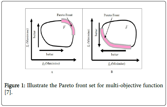
In the single objective particle swarm optimization the main goal is to optimize a single objective function and determine the overall optimum value for that objective. However, the definition of multiobjective particle swarm optimization is more complex. In MOPSO the main purpose is to determine a trade-offs solution which is representing the best possible compromises among the various objectives, this is called Pareto front [5]. Pareto front can be defined as a best possible solution. In other words, Pareto front is a set. This contains all the objective vectors relating to the parameter vectors that have not been dominated by any other parameter vectors [7]. However, when the parameter vectors dominated by another one this parameter vector is called remainder Figure 1A shows the Pareto front for two objectives maximization problems and Figure 1B shows the Pareto front for two objective minimization problems. The possible solutions which optimize f1 and f2 are also demonstrated in the Figure 1.
Reservoir Description Model
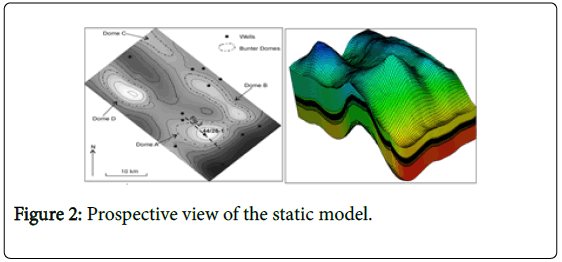
Bunter sandstone formation model from ETI UK SAP has been used as a typical saline aquifer for CO2 injection simulations. The structure of Bunter sandstone contains four domes (A, B, C, D) as shown in Figure 2 and most of these domes have been filled with saline water. Bunter model consist of five layers with alternating high and low porosity and permeability. The initial properties of Bunter formation which are used in geological model are summarized in Table 1. The detailed model of reservoir properties and characteristics of the formation are provided in Williams et al. [8].
| Properties | Unite | value |
|---|---|---|
| Bunter formation thickness | Meter | 225 |
| Permeability sandstone | mD | 0.001-15000 |
| Porosity sandstone | % | 5-35 |
| Permeability shale layer | mD | 6.5× 10⁻³ |
| Porosity shale layer | % | 3 |
| Rock compressibility | 1/MPa | 5.5675 × 10⁻⁴ |
| Temperature gradient | C°/km | 36.5 |
Table 1: Properties of Bunter formation used in the model.
Numerical simulations
Three dimensional simulations were performed using ECLIPSE 300 compositional software with CO2 STORE option that can be used to calculate mutual solubility of CO2 and brine. Bunter Model initially has a total of 110 × 63 × 65 grid blocks. Each grid measures 400 m × 400 m in X and Y directions with an average thickness of 3.9 m, the thinnest cell in the model has 0.56 m thickness. For simplicity and because of time constraint this project considered one sector of the Bunter Model (Dome A) with total of 32 × 29 × 54 grid blocks in X, Y, Z directions respectively.
For simulation input data, Viking 2 relative permeability data were used for sandstone which have been taken from SPE paper (No. 99326) published by Bennion et al. and Calmar were used for shale formation, the data have been obtained from Alberta geological survey website (AGS). The data are shown in Tables 2 and 3. In addition, because there is no specific value for fracture gradient, the fracture pressure of 0.018 Mpa/m was chosen from paper published by William et al. [8] and this vale will be used as criterion for maximum allowable pressure in injector and observation wells.
| Water Saturation Fraction | CO2 Saturation Fraction | Krg | Krw |
|---|---|---|---|
| 1.0000 | 0.000 | 0.0000 | 1.0000 |
| 0.9710 | 0.029 | 0.0002 | 0.9150 |
| 0.9420 | 0.058 | 0.0006 | 0.8332 |
| 0.9130 | 0.087 | 0.0015 | 0.7546 |
| 0.8850 | 0.115 | 0.0031 | 0.6794 |
| 0.8560 | 0.144 | 0.0055 | 0.6076 |
| 0.8270 | 0.173 | 0.0090 | 0.5392 |
| 0.7980 | 0.202 | 0.0138 | 0.4743 |
| 0.7690 | 0.231 | 0.0199 | 0.4130 |
| 0.7400 | 0.260 | 0.0276 | 0.3553 |
| 0.7110 | 0.289 | 0.0370 | 0.3014 |
| 0.6830 | 0.317 | 0.0484 | 0.2512 |
| 0.6540 | 0.346 | 0.0619 | 0.2050 |
| 0.6250 | 0.375 | 0.0776 | 0.1628 |
| 0.5960 | 0.404 | 0.0957 | 0.1248 |
| 0.5670 | 0.433 | 0.1163 | 0.0912 |
| 0.5380 | 0.462 | 0.1398 | 0.0622 |
| 0.5100 | 0.490 | 0.1660 | 0.0380 |
| 0.4810 | 0.519 | 0.1954 | 0.0190 |
| 0.4520 | 0.548 | 0.2279 | 0.0059 |
| 0.4230 | 0.577 | 0.2638 | 0.0000 |
Viking 2 Drainage data for sandstone
Table 2: Relative permeability data model for sandstone formations.
| Water Saturation Fraction | CO2 Saturation Fraction | Krg | Krw |
|---|---|---|---|
| 1.0000 | 0.000 | 0.0000 | 1.0000 |
| 0.9820 | 0.018 | 0.0039 | 0.8803 |
| 0.9640 | 0.036 | 0.0095 | 0.7697 |
| 0.9460 | 0.054 | 0.0160 | 0.6679 |
| 0.9270 | 0.073 | 0.0232 | 0.5747 |
| 0.9090 | 0.091 | 0.0310 | 0.4897 |
| 0.8910 | 0.109 | 0.0393 | 0.4128 |
| 0.8730 | 0.127 | 0.0480 | 0.3437 |
| 0.8550 | 0.145 | 0.0570 | 0.2820 |
| 0.8370 | 0.163 | 0.0664 | 0.2276 |
| 0.8190 | 0.181 | 0.0762 | 0.1800 |
| 0.8010 | 0.199 | 0.0862 | 0.1390 |
| 0.7830 | 0.217 | 0.0965 | 0.1042 |
| 0.7640 | 0.236 | 0.1070 | 0.0752 |
| 0.7460 | 0.254 | 0.1178 | 0.0518 |
| 0.7280 | 0.272 | 0.1288 | 0.0334 |
| 0.7100 | 0.290 | 0.1401 | 0.0197 |
| 0.6920 | 0.308 | 0.1515 | 0.0101 |
| 0.6740 | 0.326 | 0.1632 | 0.0041 |
| 0.6560 | 0.344 | 0.1751 | 0.0010 |
| 0.6380 | 0.362 | 0.1871 | 0.0000 |
Calmar Drainage data for shale
Table 3: Relative permeability data model for shale formations.
This study considered two cases. Case one has five injectors with one observation well while case two has seven injectors and one observation well. Initially in both cases all the wells are vertical and located around the crest of the dome A. The injector wells complete across top to the bottom aquifer and controlled by rate. However, an observation well was completed within the top three layers of the aquifer in order to monitoring pressure at the top of aquifer and minimizing the risk of formation breakdown.
In the simulation model, Dome A was divided into two regions to monitoring CO2 migration out of the dome properly. It was assumed that pure CO2 is injected into the aquifer and injection carried out for 14 years. As this study considered optimizations rather than the process occur during and after injection. Therefore, it was made some assumption to simplify the model and get shorter simulation running time. The main assumption can be summarized as the follows:
1. There are only three components in the simulation model namely; CO2, H2O and NaCl
2. Assume CO2 is the non-wetting face and ignore the effect of hysteresis by removing the keyword Hysteresis and imbibition data in the eclipse simulation
3. Because CO2 inject for 14 years so that, the mineral trapping mechanism has been ignored
4. Ignored solid precipitation
Preparing an optimization model in raven
The aim of the optimization process is to determine the parameter values that lead to a maximum or minimum of the objective function (e.g. maximum CO2 storage and minimum leakage). Therefore, before setting up the model in Raven it is important to identify the parameters that would be changed and define the range of distributions for each parameter. In this project among the relavant parameters that affect storage capacity, it was decided to change three parameters involving injection rate, well location for injector wells, and well completion. Table 4 illustrates the tuning parameters and their values that were used in the Raven software. Both cases start with 20 particles in the parameter space and run Raven for 350 iterations.
| Case one | ||
|---|---|---|
| Parameters | Well name | Range |
| Injection rate (sm3/day/well) | From I1 to I5 | 2. × 106 – 2.912×10⁶ |
| Well location in X direction | I1 | 76-79 |
| I2 | 80-94 | |
| I3 | 65-75 | |
| I4 | 76-94 | |
| I5 | 65-75 | |
| Well location in Y direction | I1 | 29-40 |
| I2 | 26-40 | |
| I3 | 22-40 | |
| I4 | 14-25 | |
| I5 | 14-21 | |
| Well completion | From I1 to I5 | 20-53 |
| Case two | ||
| Parameters | Well name | Range |
| Injection rate (sm3/day/well) | From I1 to I7 | 2 × 10⁶ - 2.912 × 10⁶ |
| Well location in X direction | I1 | 65-77 |
| I2 | 78-81 | |
| I3 | 81-94 | |
| I4 | 78-80 | |
| I5 | 65-77 | |
| I6 | 81-94 | |
| I7 | 65-77 | |
| Well location in Y direction | I1 | 25-27 |
| I2 | 29-40 | |
| I3 | 14-26 | |
| I4 | 14-25 | |
| I5 | 28-40 | |
| I6 | 28-40 | |
| I7 | 14-24 | |
| Well completion | From I1 to I7 | 20-53 |
Table 4: The ranges of parameters for case one and case two. X and Y location are given in term of grid cell number in the X and Y direction and well completion in Z direction.
Results and Discussion
Case one
Case one has five injectors and one observation well at the crest. The ranges of parameters distribution are shown in Table 3. As mentioned earlier in the single objective optimization the best solution is only one which gives minimum or maximum value of the objective. On the other hand, in the multi-objective optimization there is a set of possible solutions which is called pareto front and we are interested in determining a good compromises among the objectives that we wish to optimise. Pareto front has many advantages. For instance, it allows to decision maker (DM) to make a proper decision by noticing a wider range of solutions. From engineering point of view pareto front can also be useful because it gives a better understanding of overall system where all the consequences of a decision with respect to all objective functions can be explored.
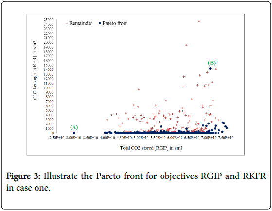
Figure 3 illustrate the pareto front for two objective problems; total amount of CO2 stored in Dome A (RGIP) and total CO2 leakage throughout Dome A (RKFR). It can be clearely seen in the trend as it moves from bottom left corner to the top right corner. This trend results from the objective function, because the objective on Y-axis is minimised and the objective on X- axis is maximised. After 352 iterations in total, fifty seven solutions for these two problems have been created as shown in blue points on Figure 3. Among these possible soutions moving from one point to another causes enhancment in one objective while the other becomes worse. In other words, each blue point which represents the possible solutions on pareto front plot is not enhanced without sacrificing performance on st leasr one other objective. For example, If the solution of the points marked (A) and (B) on the Figure 3 are compared it is clear that solution A and B are not equal for objectives RGIP and RKFR. Solution A is better for objective RKFR because it provides low leakage (3.0 sm3) compared to RKFR value in solution B which is about 14289 sm3. However, solution B is preferred over solution A for objective RGIP because it gives higher RGIP (7.1 × 10¹⁰ sm3). Similar comparison can be made for any other solutions.
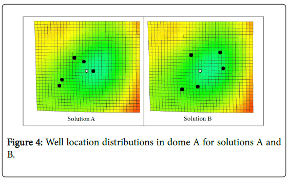
In Figure 4 it is interesting to note that the injectors (black circles) are not located around the crest as it is expected. In addition, despite that the injection rate per well in both cases are approximately the same (Table 5), the total CO2 storage in solution B is increased by factor 2.3 compared to solution A. There are two possible reasons for this, first it may be due to the problem of pressure build up in solution A as can be observed from Figure 4. The Injector wells are placed close to each other and because these wells are operated at BHP of 210 bar, a small amount of CO2 have been injected. Consequently, a small amount of CO2 migrates throughout the dome A (Table 5). The second reason is that, it could be due to the effect of permeability because Bunter formations are very heterogeneous [8].
| Parameters | Well name | Value | |
|---|---|---|---|
| Solution A | Solution B | ||
| Injection rate (sm3/day/well) | I1 | 2093721 | 2056742 |
| I2 | 2362111 | 2344729 | |
| I3 | 2115028 | 2267649 | |
| I4 | 2369112 | 2356712 | |
| I5 | 2296472 | 2115469 | |
| Well location in X direction | I1 | 71 | 80 |
| I2 | 78 | 83 | |
| I3 | 82 | 86 | |
| I4 | 72 | 75 | |
| I5 | 75 | 75 | |
| Well location in Y direction | I1 | 21 | 25 |
| I2 | 29 | 28 | |
| I3 | 26 | 22 | |
| I4 | 23 | 23 | |
| I5 | 30 | 28 | |
| Well completion | I1 | 28 | 34 |
| I2 | 25 | 27 | |
| I3 | 30 | 51 | |
| I4 | 25 | 44 | |
| I5 | 27 | 32 | |
Table 5: The parameters value for solution A and B in case one.
When several possible solutions are available, it becomes difficult to make the appropriate or best decision without having proper information and some engineering criterion. With regard to CO2 leakage, the research carried out by Zwaan et al. [9] confirmed that the acceptable leakage rate is about 0.1%/year and if the leakage rate high than this value it does not consider as a mitigation option. Therefore, it was assumed that the criterion of 0.1% is the maximum allowable leakage throughout dome A.
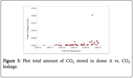
Figure 5 is the plot between total amount of CO2 stored in dome A vs total CO2 leakage during 14 years of injection for the above fifty seven solutions (Figure 4). Although there are different values for leakage, these values never exceeded 0.1% which was set as a constrained for maximum leakage in dome A. The maximum value for CO2 leakage is 0.00203%.
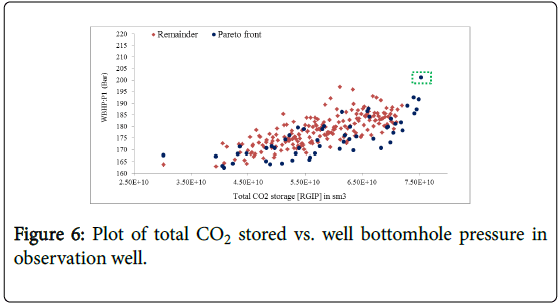
Pressure build-up was also considered in case one. Figure 6 shows the plot of total amount of CO2 stored (RGIP) against well bottomhole pressure in observation well (WBHP: P1). The goal here is to maximize storage capacity and minimize pressure build up. As depicted in Figure 6 the solutions (blue points) are widely spread because in objective WBHP the optimizer tend to determine the smallest value, but due to conflicting objectives of RGIP and WBHP there are a continuous spread of the results for all subsequent iterations. Also 350 iterations may not be enough to see convergence, because study on MOPSO performance indicates that the objective function at early stage of evaluation is decreased while flattened later on. Thus, if the number of iterations increases, the front is clearly seen as a line at shallower right corner. Generally one of the purposes of optimization injection design is to ensure that the pressure never exceeds the fracture pressure of the aquifers. Considering that the fracture pressure of Bunter sandstone is 0.018 Mpa/m, 200 bars was set as the maximum bottomhole pressure in well P1. After 352 iterations and among fifty seven solutions only one solution which is highlighted in green has reached the criterion, but the rest are below the maximum pressure limit. This is shown in Figure 6.
In Figure 7 the objective problems of well bottom-hole pressure for observation well and CO2 leakage are compared and since the objectives are minimized the trend moves from right to the left. For this case let’s compare solutions of point C and D as shown on Figure 6. Despite both solutions C and D in Pareto dominance condition are true, point C is better for both objectives than D, because it records the minimum value for both objectives. Therefore, it can be said that solution C dominates solution D. In other words, solution C is not worse than solution D for both objectives or solution C is better than solution D for at least one objective.
Case two
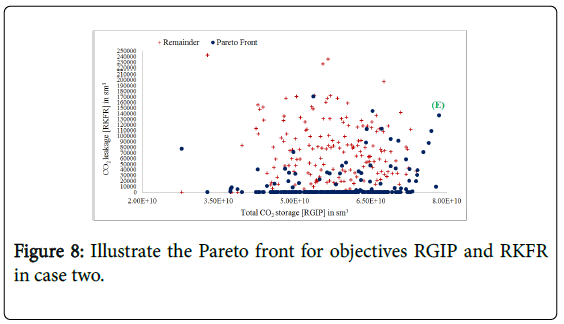
Case two has seven injector wells with one observation well. Similar to case one three parameters have been changed and the range of these parameters are illustrate in Table 4. After initializing Bunter model, 352 iterations in total were launched and fifty seven solutions have been generated. Figure 8 once again shows the plot for objectives of the total CO2 storage and total CO2 leakage rate. In contrast to case one the Pareto front (blue points) in case two as shown in Figure 8 are more scattered and it has no clear convergence trend as a line, but the front can be observed. However, because case two has two more injectors it provides more CO2 stored in Dome A for the same period of injection (14 years) compared to case one. The maximum CO2 storage for case two which has been marked (E) on Figure 8 is 3.1 × 10⁹ sm3 higher than case one. At the same time, it also gives higher CO2 leakage (1.3 × 10⁵ sm3) compared to case one which is about 1117 sm3.
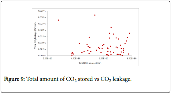
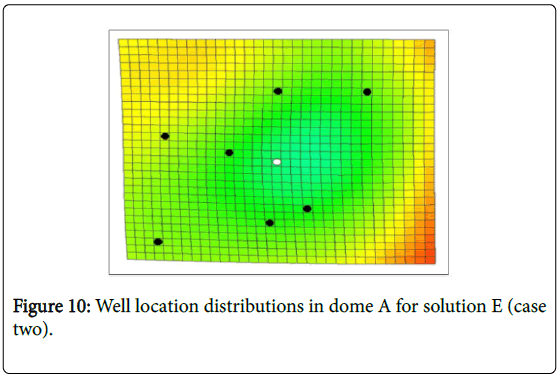
Figure 9 shows the CO2 migration throughout Dome A in percentage for above fifty seven solutions vs. total CO2 storage. In Figure 9, maximum CO2 leakage is about 0.032% and this value is 0.0299% higher than the maximum value in case one (0.00203%). Looking into the well distribution in Figure 10 it is realized that the relatively large amount of CO2 leakage in case two compared to case one result in the well locations since some injectors (black circles) being closer to the boundary. Despite the fact that the total CO2 storage and total CO2 leakage in case two is higher than case one, interestingly, case two is still under the leakage constraint (0.1%/year). Thus, to find the maximum safe volume of CO2, extended injection period are required.
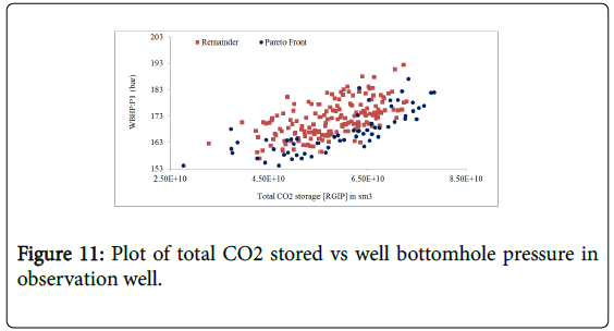
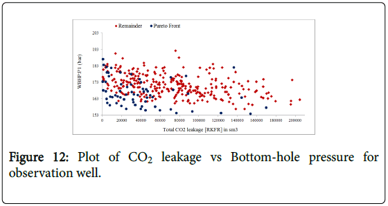
A look at Figure 11 reveals that MOPSO algorithm provides a closer front of solutions toward right corner of the plot. This result indicates an improvement in Pareto front for well bottomhole pressure compared to case one where the front widely spread. Again even with injecting more CO2 in case two, it can be seen from Figure 11 that WBHP is still lower than the maximum pressure limit (200 bar). Finally, Figure 12 shows two minimize objectives WBHP and RKFR. On the contrary to case one (Figure 7), a strong trend towards better quality value in both objectives is evident.
Concluding Remarks
In this project the optimization of CO2 storage in one sector of Bunter Model (Dome A) has been investigated by applying MOPSO algorithm with the objectives of maximizing CO2 storage, minimizing pressure build-up and CO2 leakage. The following are the conclusions derived from this study:
• This study shows that the MOPSO algorithm worked well and efficiently to optimize various parameters in the project of CO2 storage
• Possible storage capacity in case one was 139 Mt. This result shows that more CO2 could be injected
• When added two more injectors in case two the possible storage capacity for Dome A was increased from 139 Mt to 145 Mt
• Results indicate that even with increasing storage capacity by 4.1% in case two, the maximum CO2 leakage did not reach the criterion of 0.1%/year. To determine the maximum safe volume of CO2 further extended CO2 injection are required
• Based on the optimization results, well bottom-hole pressure in observation well for both cases never exceeds the fracture pressure of the Bunter formation. However, in case one (solution A) pressure build-up in adjacent well cause to reduction storage capacity by factor 2.3
Further work
Future work needs to be carried out on optimization number of wells by applying one of those algorithm methods that are available in Raven software.
It is recommended that further work on optimization study be performed using differential evolution and Bayesian optimization algorithms and needs to be compared with the results of the current study in order to know which methods give better results.
Acknowledgements
The financial support for this work was provided by Kurdistan Regional government which is gratefully acknowledged. I would also like to thank Dr. Gillian E. Pickup, Dr. Dan Arnold and Dr.Vasily Demyanov for their expert guidance throughout the tenure of this work. I additionally acknowledge the Heriot Watt University for providing Computational resources used in this work.
References
- Jin M, Mackay EJ, Quinn M, Hitchen K, Akhurst M (2012) Evaluation of the CO2 Storage Capacity of the Captain Sandstone Formation, SPE Europec/EAGE. Annual Conference, Copenhagen, Denmark 1-15.
- Mo S, Zweigel P, Lindeberg E, Akervoll I (2005) Effect of geological parameters on CO2 storage in deep saline aquifers, SPE Europec/EAGE annual Conference, Madrid, Spain 1-8.
- Orr FM (2004) Storage carbon dioxide in geological formation, SPE 88842, distinguished author series 90-97.
- Zhang Z, Agarwal RK (2013) Numerical simulation and optimisation of CO2 sequestration in saline aquifers for enhanced storage capacity and secured sequestration', International Journal of Energy and Environment 4: 387-398.
- Delshad M, Wheeler MF, Kong X (2010) A critical assessment of CO2 injection strategies in saline aquifers, SPE Western Regional Meeting, California, USA 1-18.
- Poil R, Kennedy J, Blackwell T (2007) Particle swarm optimisation, Swarm intell 1: 33-57.
- Ngatchou P, Zarei A, El-Sharkawi MA (2005) Pareto multi objective optimisation, 13th International Conference on Intelligent Systems. Application to Power Systems, Arlington 84-91.
- Williams JDO, Jin M, Bentham M, Pickup GE, Hannis SD, et al. (2013) Modelling carbon dioxide storage within closed structures in the UK Bunter Sandstone Formation', International Journal of Greenhouse Gas Control 18: 38-50.
- Zwaan B, Smekens K (2009) CO2 capture and storage with leakage in an energy-climate model, Environ model assess 14: 135-148.
Relevant Topics
- Aquatic Ecosystems
- Biodiversity
- Conservation Biology
- Coral Reef Ecology
- Distribution Aggregation
- Ecology and Migration of Animal
- Ecosystem Service
- Ecosystem-Level Measuring
- Endangered Species
- Environmental Tourism
- Forest Biome
- Lake Circulation
- Leaf Morphology
- Marine Conservation
- Marine Ecosystems
- Phytoplankton Abundance
- Population Dyanamics
- Semiarid Ecosystem Soil Properties
- Spatial Distribution
- Species Composition
- Species Rarity
- Sustainability Dynamics
- Sustainable Forest Management
- Tropical Aquaculture
- Tropical Ecosystems
Recommended Journals
Article Tools
Article Usage
- Total views: 10993
- [From(publication date):
December-2015 - Apr 04, 2025] - Breakdown by view type
- HTML page views : 9976
- PDF downloads : 1017

