Monitoring the Land Surface Temperature and Its Correlation with NDVI of Chiniot by Using GIS Technology and Remote Sensing
Received: 29-Apr-2022 / Manuscript No. jescc-22-57764 / Editor assigned: 02-May-2022 / PreQC No. jescc-22-57764 (PQ) / Reviewed: 16-May-2022 / QC No. jescc-22-57764 / Revised: 20-May-2022 / Manuscript No. jescc-22-57764 (R) / Accepted Date: 20-May-2022 / Published Date: 27-May-2022 DOI: 10.4172/2157-7617.1000621
Abstract
The unplanned and rapid increased in urban area have changed the atmospheric conditions and the non-urban area have less warm as compare to urban areas. In study area little portion of Chenab River include and the river bed contains the sand it shows high temperature value due to its specific heat energy. For this study Landsat-5 (February 2000), Landsat-7(February 2005, 2010) and Landsat-8 (Feb 2015, Feb 2020, Feb 2022) acquired from USGS. The LST and NDVI correlation is negative and it is clearly seen that in the analysis of Landsat-8 (OLI/TIRS) the Land Surface Temperature is increases 3.5408oC from 2015 to 2022. The analysis of Landsat-7(ETM+) the Land Surface Temperature is increases 3.3461oC from 2005 to 2010. In the Correlation analysis (LST&NDVI) the most of vegetation occurs between 11oC to 28oC.
Keywords: GIS; Remote sensing; LST; NDVI; Landsat-8, Climate change, Correlation
Keywords
GIS; Remote sensing; LST; NDVI; Landsat-8, Climate change, Correlation
Introduction
The Land Surface Temperature (LST) is that the radiative skin temperature of the land surface, as measured within the direction of the remote device. It’s likely from Top-of-Atmosphere brightness temperatures from the infrared spectral channels of a constellation of fixed satellites. Its estimation additional depends on the ratio, the vegetation cover and also the soil wet. LST may be a mixture of vegetation and bare soil temperatures [1-4]. As a result of each respond apace to changes in incoming radiation thanks to implementers and aerosol load modifications and variation of illumination, the LST displays fast variations too. In turn, the LST influences the partition of energy between ground and vegetation, and determines the surface air temperature [1-4].
Over the past many decades in Remote Sensing community, land surface temperature (LST) is found to be one among the foremost necessary parameters within the physical processes of surface energy and water balance at native through world scales [5]. In additional general terms LST are often outlined as hotness of surface of earth, from RS satellite’s perspective, the surface is no matter it sees once it's through the atmosphere to the bottom. LST estimation provides information concerning temporal and spatial variations of the surface equilibrium state and is of basic importance in several applications. LST is getting used in an exceedingly type of areas like evapotranspiration, climate change, hydrological cycle, vegetation watching, urban climate and environmental studies, among others [6,7] Since the launch of the Landsat-8 satellite (also referred to as Landsat knowledge Continuity Mission, LDCM) in Feb 2013 continuity of remote sensing knowledge at high spatial resolution non heritable by instruments on board previous Landsat satellites like the multispectral scanner system (MSS), the thematic mapper (TM), and therefore the increased thematic plotter and (ETM+).
Normalized distinction Vegetation Index (NDVI) quantifies vegetation by measurement the distinction between near-infrared (which vegetation powerfully reflects) and red light (which vegetation absorbs). NDVI continually ranges from -1 to +1. However there isn’t a definite boundary for every kind of land cover. For instance, after you have negative values, it’s extremely seemingly that it’s water. On the opposite hand, if you've got associate NDVI worth on the brink of +1, there’s a high chance that it’s dense inexperienced leaves. However once NDVI is on the brink of zero, there aren’t inexperienced leaves associated it may even be an urbanized space. The result of this formula generates a value between -1 and +1. If you have low reflectance (or low values) in the red channel and high reflectance in the NIR channel, this will yield a high NDVI value, and vice versa. Overall, NDVI is a standardized way to measure healthy vegetation. When you have high NDVI values, you have healthier vegetation. When you have low NDVI, you have less or no vegetation.
Landsat 5 carried the same instruments, including the Thematic Mapper and Multi-Spectral Scanner. The Multi-Spectral Scanner was powered down in 1995, but reactivated again in 2012. Landsat 7 has a solid-state memory of 378 G bits (roughly 100 images). The main instrument on board Landsat 7 is the Enhanced Thematic Mapper Plus (ETM+), a whisk broom scanner image sensor Landsat 8 is an American Earth observation satellite launched on 11 February 2013. It is the eighth satellite in the Landsat program; the seventh to reach orbit successfully. Originally called the Landsat Data Continuity Mission (LDCM), it is collaboration between NASA and the United States Geological Survey (USGS). NASA Goddard Space Flight Center in Greenbelt, Maryland, provided development, mission systems engineering, and acquisition of the launch vehicle while the USGS provided for development of the ground systems and will conduct ongoing mission operations. It comprises the camera of the Operational Land Imager (OLI) and the Thermal Infrared Sensor (TIRS) which can be used to study Earth surface temperature and is used to study global warming. The satellite was built by Orbital Sciences Corporation, who served as prime contractor for the mission. The spacecraft's instruments were constructed by Ball Aerospace & Technologies and NASA's Goddard Space Flight Center (GSFC), and its launch was contracted to United Launch Alliance (ULA). During the first 108 days in orbit, LDCM underwent checkout and verification by NASA and on 30 May 2013 operations were transferred from NASA to the USGS when LDCM was officially renamed to Landsat 8.
Study Area
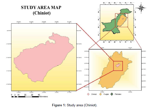
Chiniot is that the thirty sixth district of Punjab province Pakistan Located on the bank of the river Chenab, it is the 28th largest city of Pakistan. It’s given the standing of district in 2009 [8- 13]. Major a part of the district consists upon the agricultural areas and their basic supply of financial gain is agriculture. The folks of villages square measure un-educated and have lack of awareness. Chiniot comprises a collection of many tiny villages and cities. Villages square measure commonly "Chak No” whereas Chiniot town contains of redundant Municipal Committee (MC) Chiniot out of total 44 Union Councils (UC) within the Chiniot district, eight Urban UC area unit comprised in Chiniot town. Chiniot town had a population of 251,671 in 1998 that accumulated up to 314,917 in 2017; the population in Chiniot for 2021 is 222,525. In the last national census of Asian country and it's being expected that population of Chiniot can become 0.4 million in 2030 (PMSIP, 2009). Chiniot is located within the Northwest of canal Chenab. It’s coupled with the most cities of Punjab, like city, Faisalabad, Sargodha and Jhang via roads. It is 160 km distant from city to the east, concerning thirty km from metropolis to south-west, concerning 56 km from Sargodha to the west and 86 km from Jhang to south-west. Chiniot is found at latitude of 31°43ʹ to 31°44ʹ North latitude and 72°58ʹ to 73°0ʹ East great circle on the world as shown Figure 1.
Methodology
NDVI
NDVI is used to quantify vegetation greenness and vegetation density as well as plant health. NDVI is calculated as a ratio between the red (R) and near infrared (NIR) values. Download the data from the USGS, and then import the raster image into the ArcMap. Open the ArcMap toolbox called spatial analysis tool open it then select map algebra then open the raster calculator, here we can write the mathematical equation: (NIR - R) / (NIR + R).
For LandSat-7&5: Band4 subtract form Band3 and then divide it with Band4 Add Band3

For LandSat-8 Band 5 subtract form Band 4 and then divide it with Band5 Add Band 4

Land surface temperature (LST) of Landsat 5& 7
First download the Landsat-7 image from USGS then import the thermal band (Band 6 is the thermal band in the Landsat-7) in ArcMap. Then Convert the Digital Number (DN’s) into the radiance by using the following equation;
Radiance can be computed by using this formula Lλ = ML x Qcal + AL
Surface temperature was computed from the Top of Atmosphere radiance image using the formula,

Similarly, for Landsat TM, TOA radiance in Wm-2Sr-1, was computed using the formula,
Lλ = (Lmaxλ – Lminλ)/ QCALmax – QCALmin x (DN – QCALmin) + Lminλ
While the surface temperature from the computed radiance is given by

The computed temperature in Kelvin scale was converted to Celsius scale using the relationship,

Where,
L =Spectral radiance
QCAL = Quantized calibrated pixel value in DN
LMAX = Spectral radiance scaled to QCALMAX in (Watts/ (m2 • sr • μm))
LMIN = Spectral radiance scaled to QCALMIN in (Watts/ (m2 • sr • μm))
QCALMIN = Minimum quantized calibrated pixel value (corresponding to LMINA)
QCALMAX = Maximum quantized calibrated pixel value (corresponding to LMAX,) in DN= 225
Where,

Land surface temperature (LST) of Landsat 8
The Land Surface Temperature is calculated by the Landsat 08 thermal bands (band 10 and band 11). We applied a group of equations through a raster image calculator in ArcMap.
Calculation of Top of Atmospheric (TOA) spectral radiance:
The top of Atmosphere can be calculated by using the following formula

The vales of ML and AL are got from the MLT file.
Where;
ML = Band-specific multiplicative rescaling factor from the metadata Qcal = corresponds to band 10 and band 11
AL = Band-specific additive rescaling factor from the metadata.
TOA to Brightness Temperature conversion:

K1 = Band-specific thermal conversion (constant'
K2 = Band-specific thermal conversion (constant) L = Top of Atmosphere
Calculate the mean of band 10 and band 11 BT by using a tool called Cell Statistics. (Calculate mean value).
Calculate the NDVI:

Calculation of the NDVI is important because, subsequently, the proportion of vegetation (Pv), which is highly related to the NDVI, and emissivity (ε), which is related to the Pv, must be calculated.
Calculate the proportion of vegetation Pv:

Calculate Emissivity ε:
The value of 0.986 corresponds to a correction value of the equation.
ε = 0.004 * Pv + 0.986
Calculate the Land Surface Temperature:
Apply the LST equation to obtain the surface temperature Map.

| SENSOR | CONSTANT 1 – KT (WATTS/(M2 * SR * UM)) | CONSTANT 2 - K2 KELVIN |
|---|---|---|
| LANDSAT-7 ETM+ | 666.09 | 1282.71 |
| LANSAT -5 TM | 607.76 | 1260.56 |
Table 1: Spectral radiance.
Correlation LST & NDVI
Add the image into ArcMap who NDVI and LST is calculated, then apply the tool (Create fishnet). Create Fishnet is completely run then use the tool (Extract Multi Values to point) on both images (LST & NDVI) then clip tool is used on the output which generates in the result of Extract Multi Values to point. Open the attribute table of clip image here two new fields are created one is NDVI other one is LST. Go to Create Graph option select scatter plot, on x-axis assign LST and on y-axis assign NDVI click on next. Finally Correlation graph of LST & NDVI is created.
Result
NDVI
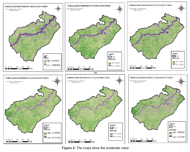
The result of NDVI of February 2000 shows the maximum value is 0.04186 and the minimum value is -0.0666. The result of second Image of NDVI (funerary 2005) shows the maximum a value is 0.5882 and the minimum value is -0.0769. The result of third image of NDVI (February 2010) shows the maximum value is 0.7108 while the minimum value is -0.1184. The result of fourth image of NDVI (February 2015) shows the maximum value is 0.4839 and the minimum value -0.1313. The result of fifth image of NDVI (February 2020) shows the maximum value is 0.5024 and the minimum value -0.1467.The result of sixth image of NDVI (February 2022) shows the maximum value is 0.5393 and the minimum value -0.1375. Day by day built-up Area is increases and the area for crop production and green space decreases. The area of snow, barren land, sand shows the very low NDVI values (For example 0.1 or less) in the maps its clear see the area around the river and builtup there is no vegetation its value is less than 0.1. Sparse vegetation (senescing crops, grasslands, shrubs) it shows the NDVI from 0.2 to 0.5.High value of NDVI is 0.6 to 0.9 in the forest region or when the crops at peak growth stage. In February 2010 the crops are at peak growth stage shows the 0.7108. The Climate is also change in February 2010 the crops is at their peak growth stage while in 2022 the crops show the moderate value i.e. 0.5393 (as shown in Figure 2).
Land Surface Temperature
The first analysis of (Landsat-5) February 2000 shows the maximum high land surface temperature is 34.0663oC and the minimum land surface temperature detect by the sensors are 10.4435oC. The second Analysis of February 2005(Landsat-7) shows the maximum high land surface temperature is 31.1872oC and the minimum land surface temperature is 9.8375oC. The third Analysis of February 2010(Landsat-7) shows the maximum high temperature is 34.5333oC and minimum land surface temperature is 11.594oC. The change in land surface temperature from February 2000 to February 2005 is 2.8758oC (decrease) and the change in land surface temperature from February 2005 to February 2010 is 3.3461oC (increase as shown in Figure 3).
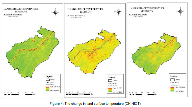
The fourth analysis of (Landsat-8) February 2015 shows the maximum high land surface temperature is 31.4826oC and the minimum land surface temperature detect by the sensors are 15.1603oC.
The fifth analysis of (Landsat-8) February 2020 shows the maximum high land surface temperature is 32.0681oC and the minimum land surface temperature detect by the sensors are 8.1522oC. The sixth analysis of (Landsat-8) February 2022 shows the maximum high land surface temperature is 35.0234oC and the minimum land surface temperature detect by the sensors are 9.5734oC. The change in land surface temperature from February 2015 to February 2020 is 0.5855oC (increase) and the change in land surface temperature from February 2020 to February 2022 is 2.9553oC (increase) as shown in Figure 4.
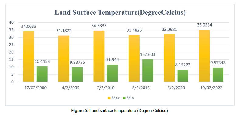
The red line indicates high temperature value there is actually river bed made-up of sand. As sand absorb maximum heat due to specific heat energy (the amount of energy needed to rise the temperature of an object) in this case sand receiving its energy from the sun. Sand has very low specific heat energy as compare to water, so sand get rapidly warm from sunlight and rapidly cool in the absence of sunlight (As shown in Figure 5).
On y-axis temperature show in degree Celsius while on x-axis shows the date of satellite image on which the LST analysis is perform. It is clearly seen that the LST increases.
Correlations of Land Surface Temperature and Normalized Difference Vegetation
Index
The Analysis of Landsat-5(TM) February 2000 the correlation of land surface temperature and normalized difference vegetation index show the trend between 11.529oC to 18.24oC. The Analysis of Landsat- 7(ETM+) February 2005 the correlation of land surface temperature and normalized difference vegetation index show the trend between 21.532 to 26.21oC. The Analysis of Landsat-7(ETM+) February 2010 the correlation of land surface temperature and normalized difference vegetation index show the trend between 21.642oC to 29.027oC (as shown in Figure 6) (Table 2).
| DATA SOURCE & DATAED | LAND SURFACE TEMPERATURE | NORMALIZED DIFFERENCE VEGETATION INDEX | |||
|---|---|---|---|---|---|
| DATA SOURCE | DATE | MAX | MIN | MAX | MIN |
| LANDSAT-5 | 17/02/2000 | 34.0633 | 10.4453 | 0.4186 | -0.0666 |
| LANDSAT-7 | 04/2/2005 | 31.1872 | 9.83755 | 0.5882 | -0.0769 |
| LANDSAT-7 | 02/2/2010 | 34.5333 | 11.594 | 0.7108 | -0.1184 |
| LANDSAT-8 | 08/2/2015 | 31.4826 | 15.1603 | 0.4839 | -0.1313 |
| LANDSAT-8 | 06/2/2020 | 32.0681 | 8.15222 | 0.5024 | -0.1467 |
| LANDSAT-8 | 19/02/2022 | 35.0234 | 9.57343 | 0.5393 | -0.1375 |
Table 2: Correlations of Land Surface Temperature and Normalized Difference Vegetation Index.
The Analysis of Landsat-8(OLI/TIRS) February 2015 the correlation of land surface temperature and normalized difference vegetation index show the trend between 15.982oC to 20.506oC. The Analysis of Landsat-8(OLI/TIRS) February 2020 the correlation of land surface temperature and normalized difference vegetation index show the trend between 16.089oC to 17.649oC. The Analysis of Landsat- 8(OLI/TIRS) February 2022 the correlation of land surface temperature and normalized difference vegetation index show the trend between 18.201oC to 12.307oC. It indicates that the most of vegetation occurs where the land surface temperature between 11oC to 27oC (as shown in Figure 7).
Conclusion and Discussion
Land surface temperature is an important variable with in the earth climate system. The land surface temperature increases due to change in climate Change and urban sprawl. In this study Landsat5, Landsat7 & Landsat-8 data is acquired from United States Geological Survey (USGS). The urban area shows the high values of LST as compare to vegetation area. The analysis of Landsat-7(ETM+) show that the Land Surface Temperature is increases 3.3461oC from 2005 to 2010. In February 2010 the crops are at peak growth stage shows the 0.710(NDVI) while in 2022 the crops show the moderate value i.e. 0.5393(NDVI) The analysis of Landsat-8(OLI/TIRS) the Land Surface Temperature is increases 3.5408oC from 2015 to 2022. The changed and unchanged bare land and built-up area suffer from the increasing trend of land surface temperature and it significantly present the influence in the climate change. The main objective of present study was to detect the changes in vegetation cover and land surface temperature due to urbanization in Chiniot area. The value of NDVI and LST was obtained for the years of 2000, 2005, 2010, 2015, 2020 and 2022. In this study; it is found that the correlations between LST and vegetation depend on the season-of-year and time-of-day. For winter or cold season, the correlation between NDVI and LST and regression coefficient from NDVI to LST are positive. The strong negative correlation between LST and NDVI is only found in the warm months from May to October. The increases in NDVI lower daytime LSTmax and daily mean LST during spring, summer, and fall. The cooling effect of vegetation on LST is much stronger during daytime (LSTmax) than nighttime (LSTmin). Thus the hypothesis for temperature-related drought indices might only be true for warm seasons. During summer, the negative correlations between NDVI and the daily mean LST are much stronger than those between NDVI and the brightness temperature from this aspect, using daytime LST for drought monitoring should be more reasonable than using brightness temperature. Further investigations about using daytime LST derived from GOES for drought monitoring will be developed in a future work.
References
- Yeang K, Richards I (2007) Eco Skyscrapers. Images Pub.
- Brunsell NA, Gillies RR (2003) Length scale analysis of surface energy fluxes derived from remote sensing. J Hydrometeorol 4(6):1212–1219.
- Karnieli A et al (2010) Use of NDVI and land surface temperature for drought assessment limitations. J Clim 23(3):618-633.
- Kustas W, Anderson M (2009) Advances in thermal infrared remote sensing for land surface Modeling. 12(4):2071–2081.
- Kalma JD (2008) Estimating land surface evaporation: a review of methods using remotely sensed surface temperature data. 29(4):421–469.
- Arnfield AJ (2003) Two decades of urban climate research: a review of turbulence, exchanges energy and water, and the urban heat island. 23(1):1-26.
- McDowell J (2013) Satellite Catalog. Jonathan's Space Page. Retrieved 16 June.
- Landsat 5 Solar Array Drive Anomaly (2017) USGS. Archived from the original.
- LANDSAT 7 Satellite details 1999-020A NORAD 25682 (2015). N2YO 25.
- Adrienne A (2016) NASA's Restore-L Mission to Refuel Landsat 7, Demonstrate Crosscutting Technologies. NASA.
- Susca T, Gaffin SR, Dell GR (2011) Positive effects of vegetation: urban heat island and green roofs. Environ Pollut 159(8-9), 2119–2126.
- Pettorelli N, Vik JO, Mysterud A (2005) Using the satellite-derived NDVI to assess ecological responses to environmental change. Trends Ecol Evol 20(9):503-510.
- Choi H, Lee W, Byun W (2012) Determining the effect of green spaces on urban heat distribution using satellite imagery. Asi J Atmo Environ 6(2):127- 135.
Indexed at, Google Scholar, Crossref
Indexed at, Google Scholar, Crossref
Indexed at, Google Scholar, Crossref
Indexed at, Google Scholar, Crossref
Indexed at, Google Scholar, Crossref
Indexed at, Google Scholar, Crossref
Citation: Ghouri AY, Khan A (2022) Monitoring the Land Surface Temperature and Its Correlation with NDVI of Chiniot by Using GIS Technology and Remote Sensing. J Earth Sci Clim Change, 13: 621. DOI: 10.4172/2157-7617.1000621
Copyright: © 2022 Ghouri AY, et al. This is an open-access article distributed under the terms of the Creative Commons Attribution License, which permits unrestricted use, distribution, and reproduction in any medium, provided the original author and source are credited.
Share This Article
Recommended Journals
Open Access Journals
Article Tools
Article Usage
- Total views: 2428
- [From(publication date): 0-2022 - Apr 25, 2025]
- Breakdown by view type
- HTML page views: 1812
- PDF downloads: 616


