Long-Memory and Fractal Traces in KHz-MHz Electromagnetic Time Series Prior to the ML=6.1, 12/6/2007 Lesvos, Greece Earthquake: Investigation through DFA and Time-Evolving Spectral Fractals
Received: 04-Apr-2018 / Accepted Date: 16-Apr-2018 / Published Date: 24-Apr-2018 DOI: 10.4172/2157-7617.1000465
Abstract
This paper presents evidence of long-lasting and chaotic trends in one-month kHz-MHz electromagnetic disturbances collected prior to a ML=6.1 shallow earthquake (June 12, 2017, 12:28:38 GMT, 38.84° N/26.36° E, 12 km deep, 37.5 km SSE of Mytilene town, Lesvos island, Greece) recorded by a telemetric ground station (39.23° N/26.27° E) located only 44 km away from the earthquake's epicenter. All analyzed earthquake occurrences (4.0 ≤ ML< 6.1) formed tight groups in both time and space which is significant for the investigation. The analysis is implemented via detailed timeevolving sliding-window two-slope DFA and power-law analysis of 4096 samples per window allowing hidden, potentially precursory, pre-earthquake trends to emerge. The classical two-exponent DFA results support the aspect of possible pre-earthquake activity 10-12 days prior to the ML=6.1 earthquake, for the 3-10 kHz antennas (both EW-NS orientations) and the 41-46 MHz ones, by simultaneously presenting a sudden increase of a parameter calculated from the two DFA exponent data. The time evolution of the power-law fractal-analysis data indicates activity 12-13 prior to the event, however, only for the 3 kHz antennas. Hurst exponents calculated in various analysis segments indicate persistency during the main pre-earthquake activity as well as persistency-anti-persistency changes. Potential pre-seismic activity prior to two other earthquakes of ML=5.0 and ML=4.6 is investigated and discussed. The precursory activity of reported time-series is discussed.
Keywords: Fractals; DFA; Spectral fractal analysis; Fractal dimension; Radon in soil; Earthquakes
Research Outline and Significance
This paper presents scientific evidence regarding potential precursory activity prior to a strong shallow earthquake occurred in Greece (ML=6.1, June 12, 2017). The data set included electromagnetic disturbances of the kHz-MHz ranges of one-month duration recorded by a station located only 44 km away from the strong earthquake's epicenter. The seismic activity of ML=4.5 of the near area exhibited serendipitous clustering in time and space with lengthy pre-seismic periods of low activity and with the main activity in the near vicinity of the strong ML=6.1 earthquake. The methods of time-evolving sliding-window two-slope DFA and power-law analysis were utilized. The dataset, the methods and the above facts outline the significance of the research, since it is very rare (a) to address recordings of preearthquake activity at a monitoring station this close to the epicenter of a strong earthquake and (b) to utilize different well-established methods to the recordings of (a). The outcomes of the DFA indicated signal areas of potential pre-earthquake activity, in the sense that the two DFA slopes differed significantly and indicated simultaneous longlasting behavior of the emitting geo-system. The common areas of all the potential pre-seismic DFA areas indicated a two-day period of maximum precursory likelihood, 10-12 days prior to the strong ML=6.1 earthquake. The time evolution of the power-law fractal-analysis data indicated activity 12-13 prior to the main event, however, only for the 3 antennas. The confirmation of the conclusions with two methods and with data of different frequencies and orientations was deemed as very significant. The differentiations were attributed to the robustness of the DFA in comparison to the well-established technique of the timeevolving spectral fractals.
Introduction
Earthquakes are destructive natural phenomena with adverse effects for societal safety and economy. Strong, catastrophic earthquakes are a major concern not only due to their inevitable forthcoming when certain geophysical conditions are met, but also because they are still difficult to foresee [1-5]. The problem of earthquake prediction is a significant challenge among the scientific community, with several reported attempts to resolve issues related to the discovery of credible and unambiguous seismic precursors. Nowadays, there is a plethora of published papers that provide noteworthy scientific evidence regarding the preseismic nature of patterns emerging in time-series that are recorded prior to strong earthquakes [1,3,4]. In general, during the preparation of earthquakes some kind of pre-seismic activity is anticipated, especially for observations in the vicinity of regions with crust cracking and fracture [6]. The issue of forecasting earthquake is multifaceted and difficult and includes the progressive and methodical contraction of time, space and magnitude sizes in regions where strong earthquakes are expected to occur [4]. Five phases are usually recognized in regard to earthquake prediction. The first is the establishment phase where maps are generated according to the possible magnitude sizes and prediction times of approaching seismic events. The other four phases are fuzzily separated. They are divided as follows [1,4]: (a) long-term phase (prediction up to 10 years); intermediate-term phase (prediction up to 1 year); short-term phase (prediction between 3 and 36 days); immediate-term phase (prediction less than 9 hours). This division is guided by the underlying physical mechanisms leading to strong earthquakes and by the needs of the society for the reliable prediction of the occurrence of a strong earthquake [7]. An alternative perspective has been expressed [1]. According to this publication [1], the prediction of earthquakes can be categorized into the following three divisions: long-term prediction (from 10 to 100 years); intermediateterm prediction (from 1 to 10 years); short-term prediction (less than one year). The latter, albeit impressively more troublesome than the others, is acknowledged to be the most pressing need regarding societal safety, particularly in high seismicity areas. Independently, however, from the earthquake prediction categorization there cannot be found single, one-to-one links between earthquakes and abnormalities in the associated recordings [4]. The electromagnetic precursors that emerge prior to earthquakes are promising forecasting tools as they reportedly appear in wide frequency ranges from thousandths of to several and in broad forecasting time windows, sometimes, from days up to hours prior to a forthcoming earthquake [1-4].
Pre-earthquake electromagnetic precursors have been recorded by ground-based stations [1,8-74] and satellites [75-80] and they can be detected in both the laboratory and in-situ [21-24]. Regardless of the scientific efforts, the stages of the earthquake generation and progress have not yet been fully understood. A significant reason is that the knowledge of the fracture mechanisms of the crust is still restricted [1-74]. Following the views expressed [25], one ought to expect that the preparatory processes of earthquake generation are murky, and information might be hidden in the related phenomena before the final catastrophe, at various scales e.g., in geological, geochemical, hydrological and natural factors [25]. Despite the fact that this information has undeniably been acquired before certain earthquakes, the nature of the associated observations is serendipitous [2,4] and sometimes unexpected. On the other hand, as aforementioned, it is assured that clear ULF, kHz and MHz, evident, or hidden irregularities are detected prior to destructive earthquakes over periods extending from some days to a couple of hours [4,8-25,31-35,40-42,44,48-52,58], albeit each earthquake is distinct and unfolds on a large scale. The main idea is that the principal electromagnetic transmitters are the ionic bonds within the earth's crust [1,4,22-25,37,40,41] and that their tectonic displacement is the source of electromagnetic irregularities from the hypocenters of earthquakes [1,4]. As reported by several publications [8-74], during the preparation of earthquakes, the principal electromagnetic transmitters break apart while batches of dynamically unstable multi-cracks generate continuously new cracks and propagate in the focal area under a complex spatio-temporal underlying physical pattern. The fragment of the ionic bonds, finally, generates electromagnetic waves.
This paper focuses on the short-term electromagnetic disturbances of the kHz and MHz ranges derived by ground-station measurements in Greece. The study extends one month prior to a major shallow underwater earthquake (magnitude:=ML=6.1, latitude/longitude: 38.84° N/26.36° E, depth: 12 km, epicenter location: 37.5 km SSE of Mytilene town, day: June 12, 2017, time: 12:28:38 GMT) occurring in the vicinity of Plomarion, Lesvos island (Greece). The measurements were acquired from the monitoring ground-station of Agia Paraskevi (Latitude: 39.23° N, Longitude: 26.27° E) Lesvos island, Greece, located only 44 km away from the epicenter of the Plomarion (ML=6.1) earthquake. This serendipitous finding is very rare in the literature and should be emphasized. This station is one of the eleven electromagnetic monitoring stations that are installed along the Hellenic Arc and the Anatolian and Aegean Plates and operate continuously in Greece [41,47,48,81]. Apart from the strong ML=6.1 earthquake, all the remaining noteworthy earthquakes (4.0 = ML< 6.1) of the period occurred in a circle of 120 radius from the monitoring station and were grouped into relatively short time periods and a short distance from the Agia Paraskevi station. This rare finding is very significant since it allows for (a) the discrimination of the main event (ML=6.1) from other significant earthquakes of the period in the vicinity of the Plomarion earthquake and, simultaneously, (b) the analysis of electromagnetic data during a period of one month of low earthquake activity.
The principle sought is to investigate if long-lasting and fractal trends exist in time-evolving sections of the recorded kHz- MHz electromagnetic time-series, assessing these as potential preearthquake precursors. As explained later, these trends are investigated through the sliding-window time-evolution of the classical DFA twoexponent data and power-law spectral fractal-analysis data. The analysis shows noteworthy pre-earthquake related activity 10-12 days prior to the catastrophic Plomarion ML=6.1 earthquake. The classical twoexponent DFA data from both kHz and MHz antennas support this claim in all antenna orientations though simultaneously presenting a sudden increase of a related index. The time evolution of the power-law fractal-analysis data supports also partially the above findings. Finally, the precursory activity of all the reported time-series is discussed.
Materials And Methods
Earthquake activity
The main period of the investigation of the preseismic activity prior to the Plomarion earthquake lasted 30 days, viz., started on May 12, 2017 and ended on June 12, 2017. Note that this 30-day investigation period was followed in all the previous papers of the team [11,12,40,41,44-49] for the analysis of the preseismic electromagnetic disturbances and due to this, it was considered adequate for the present approximation as well. To study the post seismic activity, 5 more days were included in the main period, namely the days from June 12, 2017 to June 17, 2017. As mentioned in section 1, the catastrophic Plomarion earthquake occurred undersea in Lesvos island (magnitude: ML=6.1, Latitude/Longitude 38.84°N/26.36°E, depth: 12, epicenter location: 37.5 SSE from Mytilene town, June 12, 2017, 12:28:38 GMT). During the whole period of investigation, several smaller earthquakes occurred in the broad vicinity of the Agia Paraskevi station (Latitude: 39.23°N, Longitude: 26.27°E). To limit the analysis to the most significant earthquakes of the period, an arbitrary magnitude.
Threshold of ML=4.5 was set, namely only earthquakes with ML=4.5 were included in the study. Note, that this threshold was lower than the ML=5.0 one employed in all the previous papers of the reporting team [11,12,37-41,44-49]. This lower threshold was adopted so as to include more nearby earthquakes as shown in Table 1, which reports the earthquakes with magnitudes ML=4, in a radius of R=150 km from Agia Paraskevi station. The earthquakes of Table 1 are illustrated in (Figure 1). It should be emphasized that the seismic occurrences are grouped not only in time (Table 1) but also in space inside areas A and B (Figure 1). With regard to the time formations, two main groups of seismic events can be observed in Table 1. The first temporal group (events 1 and 2) occurred between 27/5/2017 and 28/5/2017 (two days duration) and the second group (events 3-5) between 12/6/2017 and 17/6/2017, viz., it included the main ML=6.1 event and the two post seismic events with ML=4. The time occurrence lag between spatial groups A and B (Table 1 and Figure 1) was 14 days and the corresponding inter-group distance was approximately 135. This is a very interesting fact, since it indicates two discrete earthquake groups which are distant in both the temporal and the spatial aspects. In addition to this, area A is only 44 km away from the monitoring station of Agia Paraskevi. This observation is very rare and should be highlighted. Indeed, it is very rare in the literature to record pre-earthquake activity at a monitoring station this close to the epicenters of a strong ML=6.1 earthquake (Event 3 and Table 1) [2,4,37]. Moreover, group A includes also one noteworthy earthquake of ML=5.2 (Event 5 and Table 1).
| Event | Date | Time | Location | Latitude Longitude | Identifier in Figure 1 |
Magnitude (ML) |
Depth (km) |
|
|---|---|---|---|---|---|---|---|---|
| (GMT) | (GMT) | (°N) | (°E) | |||||
| 1 | 27-05-2017 | 15:53:23 | 134.1 km NNE of Samos | 38.76 | 27.83 | A-Star, Green | 5.2 | 24 |
| 2 | 28-05-2017 | 11:04:59 | 127.1 km NNE of Samos | 38.71 | 27.78 | A-Circle, Yellow | 4.6 | 30 |
| 3 | 12-06-2017 | 12:28:38 | 37.5 km SSE of Mytilene | 38.84 | 38.84 | B-Star, Blue | 6.1 | 12 |
| 4 | 17-06-2017 | 03:40:37 | 31.9 km S of Mytilene | 38.88 | 38.88 | B-Circle, Blue | 4.6 | 14 |
| 5 | 17-06-2017 | 19:50:05 | 38.5 km SSE of Mytilene | 38.85 | 26.43 | B-Star, Blue | 5.2 | 12 |
Table 1: Seismic events during the analysis period (May 12/2017 to June 17/2017). Color-Schema identifier in Figure 1, according to the one of the Institute of Geodynamics of the National Observatory of Athens Area Identifiers A (near Lesvos) and B (Turkey).
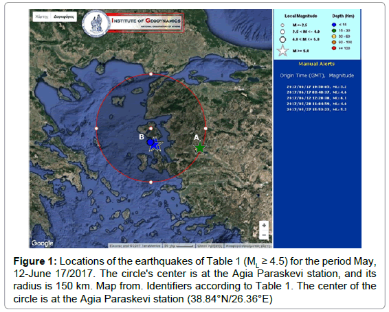
Figure 1: Locations of the earthquakes of Table 1 (ML = 4.5) for the period May, 12-June 17/2017. The circle's center is at the Agia Paraskevi station, and its radius is 150 km. Map from. Identifiers according to Table 1. The center of the circle is at the Agia Paraskevi station (38.84°N/26.36°E)
In contrary, the distance between the Agia Paraskevi station and earthquake group A was around 145 According to previous papers of the team [37-41,44-49], this group may have evoked electromagnetic disturbances to the Agia Paraskevi station. The combination, however, of the long distance and the deeper epicenter are expected to have smoothed their effect to the corresponding electromagnetic recordings.
Instrumentation
The Agia Paraskevi station is part of a telemetric network operating in Greece [11,12,37-41,44-49] which, nowadays, consists of eleven stations located at: (1) Ithomi Peloponnese, (2) Valsamata, Kefalonia Island, (3) Ioannina, (4) Kozani, (5) Komotini, (6) Agia Paraskevi, Lesvos Island, (7) Archangelos, Rhodes Island, (8) Neapolis, Crete Island, (9) Vamos, Crete Island, (10) Ileia, Peloponnese and (11) Atalanti. Stations 1, 2, 9 and 11 are located along the Hellenic Arc. Stations 5, 6, 7 are located in the vicinity of the Anatolian Plate and stations 3, 4, 8 are located in the wider area of the Aegean Sea Plate. Each station comprises (1) two electric field bipolar antennas synchronized at 41 MHz and 46 MHz; (2) two loop antennas synchronized at the frequencies 3kHz and 10 kHz and orientation East-West (EW) and North-South (NS), respectively; (3) acquisition data-loggers and (4) telemetry equipment (e.g., RF modem-wired or cordless internet).
Detrended Fluctuation Analysis (DFA)
The complex processes during the preparation of earthquakes are characterized by long-range power-law correlations and time-series with erratic fluctuations and scale-invariant behavior [55,82]. Many times, non-stationary features are embedded in the earthquake related time-series associated with pseudo sinusoidal trends [55], repeated temporal patterns [44], noise and sources of other origin. The nonstationarity of the related time-series inhibits the use of traditional methods, such as the spectrum analysis and the auto-correlation based techniques [83-85]. On the other hand, DFA has been established as an effective and robust method suitable for detecting long-range powerlaw connections in even non-stationary, noisy, randomized and short signals [39,44,53,55,71,86-91]. It has been applied with successful results to diverse fields where scale-invariant behavior emerges, such as DNA [88], heart dynamics [92,93], circadian rhythms [94] meteorology [95], climate temperature fluctuations [96], economics [97], preseismic variations of radon in soil [44] and pre-earthquake activity of SES [55,71,74], magnetic field variations [66,67,69] and electromagnetic disturbances of the MHz range [44,47]. In principle, DFA is an altered root-mean-square analysis of a random walk in view of the perception that a time signal with long-range correlations can be integrated to form a self-similar process. By calculating the scaling exponent of the integrated time series, hidden long-range associations of the original time-series can be revealed [39,44,47,88-95]. From a theoretical point of view, at first, the original time-signal is integrated. Then, the fluctuations, F(n), of the integrated signal are calculated within a time window of size. The scaling exponent (self-similarity parameter), a, of the integrated time-series is then calculatedthrough a least-square fit to the log (F(n)) - log(n) linear transformation. Depending on the scale n, the log line may display one crossover at the time scale where the slope changes abruptly. Note, that there are cases where two crossovers can be addressed [44,47] or none. The elucidation of the scaling exponents and the crossovers of the power-law behavior rely on the inherent dynamics of the system. The DFA of a one-dimensional signal yi, (i=1, N), is implemented through the following steps [39,44,47]:
First, the integrated profile of the time series is calculated according to equation (1):
 (1)
(1)
The symbol <...> denotes the overall average value of the time series and symbolizes the different time scales. The integrated signal of equation (1), y(k), is then divided into non-overlapping bins of equal length, n. In each bin of length n, y(k) is fitted to a line function which represents the trend in that box. Polynomial functions of order 2 or higher are not utilized for consistency with previous papers of the team [39,44,47]. The coordinate of the linear fit function in each box is
denoted by yn(k). The integrated signal y(k) is detrended by subtracting the local trend, yn(k), in each box of duration. In this manner, the detrended signal ydn(k)is calculated in each bin as:
 (2)
(2)
For a given bin size n, the root-mean-square (rms) fluctuations of this integrated and detrended signal is calculated as:
 (3)
(3)
Interpreting equation (3), F(n) represents the rms fluctuations of the detrended time-series ydn(k)
The above steps are iterated for a wide range of scale box sizes (n). This is done so as to provide the relationship of F(n)versus n. In general, F(n) is expected to increase with the box size n. A linear dependence between the logarithms of average root-mean square fluctuations versus the logarithms of the bin sizes (log F(n)vslog (n)) indicates the presence of long-lasting self-fluctuations:
F(n)a na (4)
The slope of line (4) is the DFA scaling exponent a which quantifies the power of the long-range correlations of the time-series.
Two different DFA implementation approaches are followed: (a) the sliding-window technique; (b) the manual DFA fluctuation-bin plot generation. Approach (a) is applied through calculation of twoslope data for windows equal or larger than 4096 samples, however, with automatic detection of the cross-over between the small and the large scales.
The steps to implement the DFA sliding window technique (a), are [39,44,47]: The signal is divided in segments-windows of 4096 size (number of samples).
In each segment, a least square fit is applied to (F(n)) - log(n) the vs representation of equation (4). Accounting for the size of the DFA boxes, one cross-over is automatically sought under the constrain that both the low and high scale fit lines exhibit squares of Spearman’s correlating coefficient above 0.95; the window is advanced one sample forward and the steps (A) and (B) are repeated until the end of the signal. Note that this one-step sliding provides fine analysis of the investigated signal under, however, the expense of high computational cost.
To apply the manual DFA fluctuation-bin plot technique, at first the time-series signal is subdivided in independent non-overlapping parts of size greater than 4096. Then in each part, a (F(n)) - log(n) plot is created. Depending on the plot, a cross-over is manually identified. Afterwards, the two slopes are calculated in terms of linear fit under the constraint of exhibiting each slope the Spearman's square correlation coefficient above 0.95. Note that this is the form of DFA that was initially introduced [89] and utilized by several researchers as well [22,39,44,53,71,74,86,87].
Fractal Analysis
As mentioned in section 2.3, during the preparation of earthquakes, the seismic systems exhibit scale-invariant behavior and long-range power-law correlations. These physical phases are associated with complex connections between space and time which produce characteristic fractal structures [25,38] as the systems evolve naturally to self-organized critical (SOC) states of spatio-temporal fractal organization [57]. The scale-invariant, long-range power-law correlations of the SOC-states fractal systems, may unfold also through the power-law fractal analysis of electromagnetic time-series of the MHz-kHz [11,12,19,23,25,31-35,37,38,40-42,44,47-49,59] and ULF [55-58] ranges.
If a time-series A(ti) is a temporal fractal, then the power spectral density (PSD), S(f) follows a power-law of the form S(f)=a·f-b, where f is the frequency of a transform. The - representation of the PSD is a straight line with slope b. The amplification quantifies the strength of the spectral components f following the power law and the spectral scaling exponent is a measure of the strength of time correlations. Note that the spectral amplification a is different from the DFA scaling exponent b. It is significant to recognize segments with distinct changes of the scaling exponent b since such changes are reported to emerge before major earthquakes [23,24,31-35,37,38,44,45,48,49,52,56-59].
In relation, the following issues are of importance [23,24,31-35,37,38,44,45,48,49,52,56-59]:
1. Scaling exponent values between b between -1 = b< 1 correspond to time-series following the fractional Gaussian noise (fGn).
2. A power-law value of b=1 means that the fluctuations of the processes do not grow, namely the associated system is stationary; Values of b in the range 1< b = 3 imply that the time-series profile is a temporal fractal and is associated with the fractional Brownian motion (fBm); Power-law values in the range 1< b< 2 imply antipersistency; A value of b=2 means that there is no correlation between process increments, viz., the system follows random paths driven by nonmemory dynamics (random-walk); Values 2< b = 3 suggest persistency of the related time-series. The accumulation of the related fluctuations is faster than in fBm modelling.
3. The fractal analysis is implemented by applying the continuous wavelet transform (CWT) with the Morlet base function in the PSD data of the investigated signals and seeking the linearity in segmented log (S(f))- log(f) fits, following previous methodology [11,12,37-41,44-49].
In specific the following steps are followed:
1. The electromagnetic time-series is divided into segments (windows). For consistency with section 2.2.1, the segmentation is set to 4096 samples per window. According to previous research [47] this segmentation reveals the fractality of the signals in a smoother manner in comparison to the usual windowing of 1024 samples per window [23,24,31-35,37,38,44,45,48].
2. In each segment the PSD of the signal is calculated. As aforementioned, the CWT with the Morlet base function is utilized.
3. In each segment the existence of a power-law of the form S(f)- a·f-b is investigated. The employed frequency is the central frequency of the Fourier transform of each Morlet scale.
4. The least square method is applied to the (S(f))- log(f) linear representation. Accurate representations are considered those that exhibit squares of the Spearman's correlation coefficient above 0.95.
Further Analysis
Fractal class segmentation
For further analysis the following two categories are formed:
Class I segments: These comprise the segments of the time-series that exhibit accurate fractal behavior (Spearman's coefficient r2 = 0.95) and simultaneously are described by the fBm class (1< b = 3). According to publications these can be classified as of noteworthy precursory value [11,12] and especially for the cases with distinct changes between high -values, namely changes between 1.7< b< 2 (anti-persistent behavior) and b>2 (persistent behavior) [37-41,44-49]. According to numerous publications [19,23,25,31-35,37,38,40-42,44,47-49] these Class I segments have been characterized as pre-earthquake footprints when the segments are very high (b>2).
Class II segments: These consist of the electromagnetic time-series portions that do not follow the prominent fBm class, viz., r2< 0.95 and 1 = b = 3, or followed the fGn class (1 = b< 1). According to several publications, these segments can be deemed of low precursory value [11,12,19,23,25,31-35,37,38,40-42,44,47-49,59]. Obviously, the Class II segments are the complement of the Class I ones [11,12].
Hurst exponent
The Hurst exponent (H) is a mathematical quantity which can indicate if a signal contains hidden long-memory patterns, namely long-range dependencies in time or space [98,99]. The Hurst exponent can be used to determine if the related physical phenomenon is a temporal fractal and can estimate the smoothness of the related timeseries [100]. The exponent was introduced initially for hydrology [98,99]. Apart from that, it has been also used in climate dynamics [101], plasma turbulence [102], astronomy and astrophysics [103], pre-epileptic seizures [104], economy [105], traffic traces [106], ULF geomagnetic fields [56,57] and pre-seismic activity [23,38,44,46]. The following are valid:
1. If the Hurst exponent is between 0.5< H < 1, the related timeseries exhibits long-lasting positive autocorrelation. This implies that a high present value will be possibly followed by a high future value and this tendency will last for long time-periods in future (persistency) [13,24,27-31];
2. If H is between 0< H< 0.5, the time-series exhibits long-term switching between high and low values. This means that a low present value will be followed by a high future value, while a high present value will be followed by a low future value. This low-high switching will continue into the future for many samples (anti-persistency) [13,24,29,31];
3. If H=0.5 the time-series profile is completely uncorrelated.
Combined calculations
As stated in several publications [39,44,47], the power-law fractal (b) and DFA (a) exponents are related as b=2·a-1 for both fBm and fGn classes, where according to section 2,3, the long-range interactions can be quantified by the DFA slopes. Since only the high b(b>1.7) Class I segments are of noteworthy precursory value (according to the papers of the reporting team [37-41,44-49]), or the fractal segments with b (according to other publications [19,23,25,31-35,37,38,40-42,44,47-49]), it can be supported that only the high DFA exponents a can be of noteworthy precursory value, as expressed in other publications [23,44,47] as well. In this manner, DFA-based power-law fractal exponents (denoted by ß) can be calculated from the long-range DFA interactions (a=a1, a2) as ß=2·a-1, considering that where the DFA slopes are relatively high, the corresponding ß values will be relatively high as well and, as aforementioned, the segment of the DFA calculations will, most probably, be of noteworthy precursory value. On the other hand, Hurst exponents can be calculated from power-law b values between 1< b = 3 (fBm class, section 2.5.1) as b=2H+1⇒H=0.5(b-1) and from power-law - values between 1< b = 3 (fGn class, section 2.5.1), as b=2H- 1⇒H=0.5(b+1) [45].
Accounting for the above facts, Hurst exponents in this paper are calculated as follows:
According to the findings of the DFA as:
H=0.5[ß-1]⇒H=0.5[(2a-1)-1]⇒H=0.5(2a-2)⇒H=0.5[2(a-1)]⇒H=a-1 (1a)
Where is the highest among and slopes under the constraints that?
1< ß = 3⇒1< 2·a-1 = 3⇒2< 2·a = 4⇒1a = 2 (1b) and as
H=0.5[ß+1]⇒H=0.5[(2a-1) +1]⇒H=0.5(2a)⇒H=a (2a)
where a=a1, a2 is the highest among a1 and a2 slopes under the constraints that:
-1 = ß< 1⇒-1 = 2·a-1< 1⇒0 = 2·a< 2⇒0 = a< 1 (2b)
According to the findings of the fractal-analysis as:
B=2H+1⇒H=0.5(b-1) (3a)
for the Class-I segments and as:
b=2H-1⇒H=0.5(b+1) (3b)
For the successive Class-II segments with 1 = b < 1. In the remaining cases the Hurst exponent values are not calculated.
Results and Discussion
As mentioned in section 1, the electromagnetic time-series of this paper were recorded by the telemetric station installed at Agia Paraskevi, Lesvos Island (Figure 1). The recording rate was 1 sample per second and due to this the whole data-set was dense. The total length of the time-series was one month, similarly to the analysis length of other papers of the team [11,12,37-41,44-49]. The onemonth data compensated between signal duration and bias due to the nearby earthquakes of (Figure 1). This is a very important fact because Greece is a country prone to seismic activity and, due to this, it is difficult to locate periods of low seismic activity. In addition, as can be recalled from section 2.1, the one-month analysis period of this paper contained, relatively, lengthy periods of low seismic activity in contrary to the significant activity of the major Plomarion ML=6.1 earthquake. The results from the application of the DFA are presented collectively in Figures 2-8, for the LF (Low Frequency) antennas recordings (kHz range) and in (Figures 9 and 10) for the HF (High Frequency) ones (MHz range). All (Figures 2-10) present the onemonth electromagnetic disturbances and the corresponding DFA slopes for the small (Slope-1, green in color figure) and the large (Slope 2, red in color figure) scales. Each figure contains DFA-slope data from the analysis of approximately 2.6 × 10⁶ discrete segments; hence, the analysis produced a great amount of DFA results. To visualize and interpret the results of DFA in each segment, Figure 11 was generated, as an example case from the data of Figure 10, however, for segments of more than 4096 samples. As can be observed from Figure 11a the large scales exhibited, for this example case (from 46 data), noteworthy high large-scale DFA slopes (Slope-2, a2=1.7884), which were significantly lower when compared to the small-scale ones (Slope-1, a1=0.79131). In contrary, (Figure 11b) shows a completely different example case (also from 46 data), where the small and the large scales did not differ much (Slope-1, a1=0.65387 and Slope-2, a2=0.78052) and the large scales did not exhibit great DFA slopes. These differentiations in the DFA slopes of (Figure 11) are characteristically shown in the area of (Figure 10a) contoured with a box (magenta in color figure) which included segments similar to the ones of (Figure 11a). In view of the described results of (Figure 10a, Figures 2-10) present an additional parameter that was calculated in every segment of each figure so as to discriminate and visualize the significant differentiations of the smallto large-scale slopes of the DFA. This parameter was named difference of DFA (hereafter referenced fference) and was calculated from the DFA slopes as
 (4)
(4)
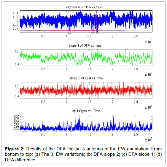
Figure 2: Results of the DFA for the 3 antenna of the EW orientation. From bottom to top: (a) The 3, EW variations; (b) DFA slope 2; (c) DFA slope 1; (d) DFA difference.
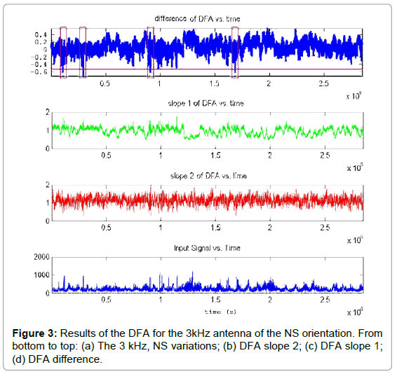
Figure 3: Results of the DFA for the 3kHz antenna of the NS orientation. From bottom to top: (a) The 3 kHz, NS variations; (b) DFA slope 2; (c) DFA slope 1; (d) DFA difference.
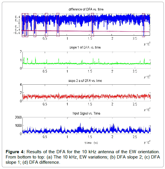
Figure 4: Results of the DFA for the 10 kHz antenna of the EW orientation. From bottom to top: (a) The 10 kHz, EW variations; (b) DFA slope 2; (c) DFA slope 1; (d) DFA difference.
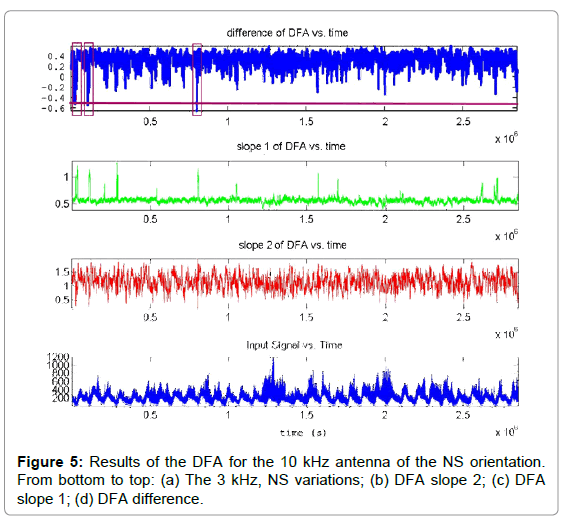
Figure 5: Results of the DFA for the 10 kHz antenna of the NS orientation. From bottom to top: (a) The 3 kHz, NS variations; (b) DFA slope 2; (c) DFA slope 1; (d) DFA difference.
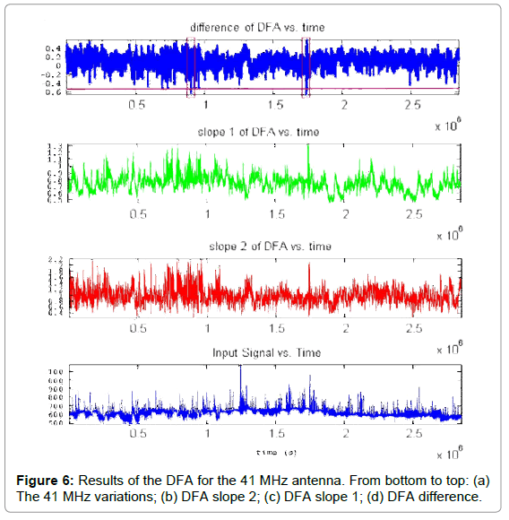
Figure 6: Results of the DFA for the 41 MHz antenna. From bottom to top: (a) The 41 MHz variations; (b) DFA slope 2; (c) DFA slope 1; (d) DFA difference.
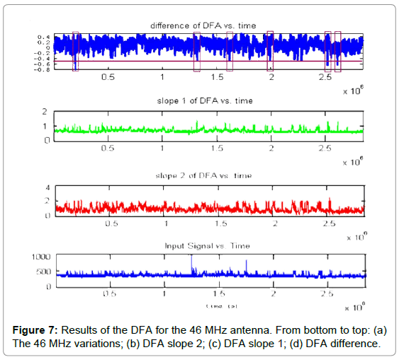
Figure 7: Results of the DFA for the 46 MHz antenna. From bottom to top: (a) The 46 MHz variations; (b) DFA slope 2; (c) DFA slope 1; (d) DFA difference.
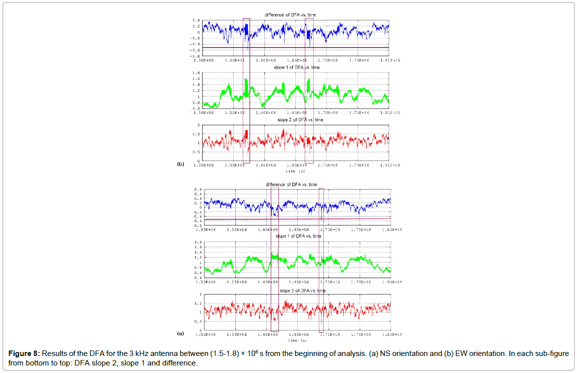
Figure 8: Results of the DFA for the 3 kHz antenna between (1.5-1.8) × 106 s from the beginning of analysis. (a) NS orientation and (b) EW orientation. In each sub-figure from bottom to top: DFA slope 2, slope 1 and difference.
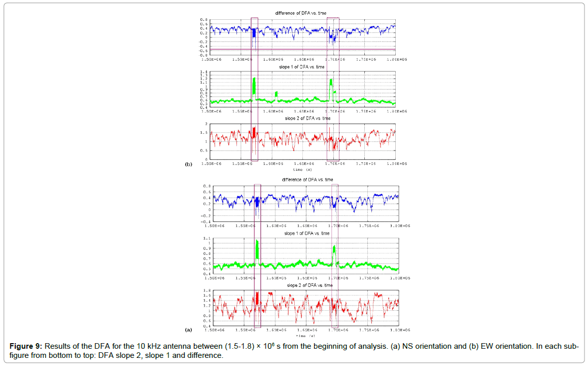
Figure 9: Results of the DFA for the 10 kHz antenna between (1.5-1.8) × 106 s from the beginning of analysis. (a) NS orientation and (b) EW orientation. In each subfigure from bottom to top: DFA slope 2, slope 1 and difference.
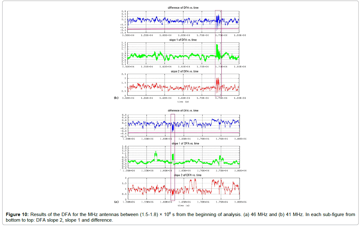
Figure 10: Results of the DFA for the MHz antennas between (1.5-1.8) × 106 s from the beginning of analysis. (a) 46 MHz and (b) 41 MHz. In each sub-figure from bottom to top: DFA slope 2, slope 1 and difference.
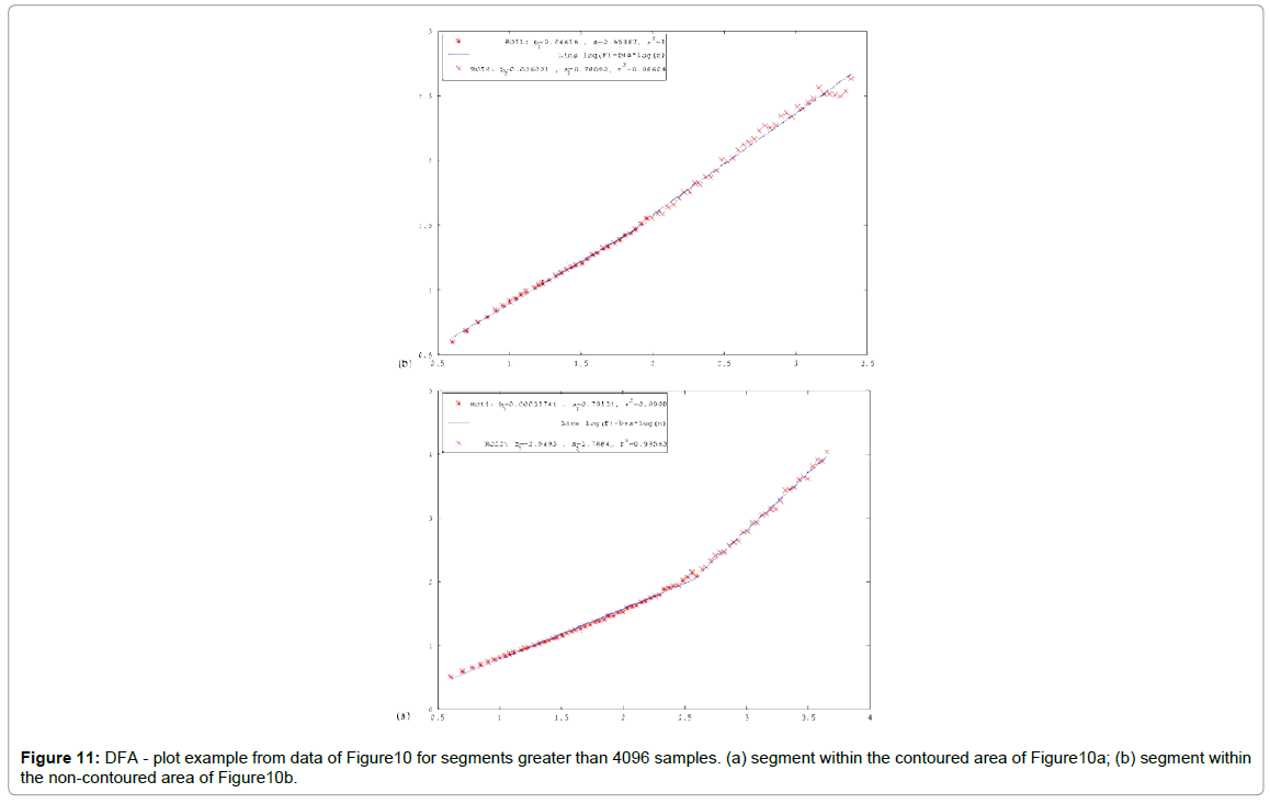
Figure 11: DFA - plot example from data of Figure10 for segments greater than 4096 samples. (a) segment within the contoured area of Figure10a; (b) segment within the non-contoured area of Figure10b.
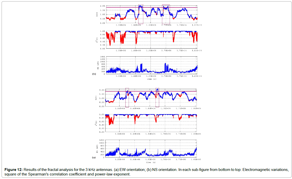
Figure 12: Results of the fractal analysis for the 3 kHz antennas. (a) EW orientation; (b) NS orientation. In each sub-figure from bottom to top: Electromagnetic variations, square of the Spearman's correlation coefficient and power-law exponent.
where i represents the segment of calculation and Slope 1, Slope 2 the DFA slopes of the small and the large scales respectively (values in colored subfigures in green and red respectively). It should be noted here that this parameter has been conceptualized from the, so called, imaging contrast, a parameter that is utilized in imaging and expresses the potentiality of an imaging system to discriminate two near pixels or areas in general. In this consensus, the DFA's difference expresses the discrimination ability between the various small-scale to large-scale DFA slopes, in the sense that where difference is high the two DFA slopes differ significantly, contrary to the areas for which the difference is average, which means that the DFA slopes are of similar measures. Especially when this parameter is viewed under the perspective of Figure 11a versus Figure 11b, it may be concluded that in the segments where the difference is significantly negative, the small DFA scales presented significantly higher slopes when compared to the one of the large scales. In a physical interpretation where the small scales are, most possibly, related to the fracture of the small areas, a significant negative difference value may be associated with the fracture of microregions, that is, the fracture of micro-cracks. Completely opposite would be the interpretation where the difference is very positive; the fracture would, most probably, refer to large areas. Most important, however, would be where the difference is significantly negative or positive and, simultaneously, both DFA slopes are high. This is because the simultaneous appearance of high and a1 and a2 values have been interpreted as a footprint of the identification of the precursory segments. When one compares the two fracture mechanisms, viz., those of the small and the big geological scales, in relation to the generation of the electromagnetic waves of the kHz-MHz ranges, it can be supported [11,12,37-42, 44-49] that the production of these waves can be attributed to the forced separation of the ionic bonds during the micro-crack generation, branching and propagation at the stages of earthquake generation, as already mentioned above. Under this perspective, of greater importance are the segments where the difference is significantly negative since these could be associated with the fracture of the micro-cracks. In this consensus, an arbitrary negative threshold was set at the difference of 0.5, so as to discriminate the most significant segments in the pre-earthquake electromagnetic time-series. Note, that this threshold implies a 50% discrepancy in the DFA slopes in the sense of equation (4). Importantly, with this threshold, all the DFA time-series, for both the LF and HF antennas and the different antenna orientations, presented areas of difference values near or below 0.5. According to the abovementioned interpretations, these areas could be of noteworthy precursory value. In the view of the above, the following detailed observations can be made from (Figures 2-10) starting the DFA from 0 or day 0, on May 12, 2017 with the main event (Event 3 and Table 1) occurring 31.5 days from day 0, namely, on May 12, 2017 (12:25 GMT, Table 1):
• (Figure 2) (3 kHz antenna, EW orientation): Three areas can be observed:
Area 1, between (1.09-1.11) × 106 S or 12.61-12.84 days from day 0, namely, between days 12-13 from day 0, viz., on May 24, 2017
Area 2, between (1.56-1.57) × 106 S or 18.05-18.17 days from day 0, namely, between days 18-19 from day 0, viz., on May 30, 2017
Area 3, between (1.67-1.68) × 106 S or 19.32-19.44 days from day 0, namely, between days 19-20 from day 0, viz., on May 31, 2017.
• (Figure 3) (3 kHz antenna, NS orientation): Four areas can be observed.
Area 1, between (0.15-0.17) × 106 S or 1.74-1.96 days from day 0, namely, between days 1-2 from day 0, viz., on May 13, 2017.
Area 2, between (0.29-0.31) × 106 S or 3.36-3.59 days from day 0, namely, between days 3-4 from day 0, viz., on May 15, 2017.
Area 3, between (0.90-0.91) × 106 or S 10.41-10.53 days from day 0, namely, between days 10-11 from day 0, viz., on May 22, 2017.
• (Figure 4) (10 kHz antenna, EW orientation): Seven areas can be observed:
Area 1, between (0.05-0.06) × 106 S or 0.57-0.69 days from day 0, namely, between days 0-1, viz., on May 12, 2017.
Area 2, between (0.10-0.12) × 106 or S 1.15-1.38 days from day 0, namely, between days 1-2 from day 0, viz., on May 13, 2017.
Area 3, between (0.32-0.34) × 106 or S 3.70-3.93 days from day 0, namely, between days 3-4 from day 0, viz., on May 15, 2017.
Area 4, between (0.53-0.55) × 106 S or 6.13-6.36 days from day 0, namely, between days 6-7 from day 0, viz., on May 18, 2017.
Area 5, between (0.82-0.83) × 106 S or 9.49-9.61 days from day 0, namely, between days 9-10 from day 0, viz., on May 21, 2017.
Area 6, between (1.55-1.57) × 106 S or 17.93-18.17 days from day 0, namely, between days 17-18 from day 0, viz., on May 29, 2017.
Area 7, between (2.72-2.73) × 106 S or 31.48-31.59 days from day 0, namely, between days 31-32 from day 0, viz., on June 12, 2017, that is, the day of the main event.
• (Figure 5) (10 kHz antenna, NS orientation): Three areas can be observed:
Area 1, between (0.15-0.17) × 106 S or 1.74-1.96 days from day 0, namely, between days 1-2 from day 0, viz., on May 13, 2017.
Area 2, between (0.29-0.31) × 106 S or 3.36-3.59 days from day 0, namely, between days 3-4 from day 0, viz., on March 15, 2017.
Area 3, between (0.85-0.86) × 106 S or 9.83-9.95 days from day 0, namely, between days 9-10 from day 0, viz., on May 21, 2017.
• (Figure 6) (41 MHz antenna): Two areas can be observed:
Area 1, between (0.86-0.88) × 106 S or 9.95-10.18 days from day 0, namely, around day 10 from day 0, viz., on May 22, 017.
Area 2, between (1.74-1.75) × 106 S or 20.13-20.25 days from day 0, namely, around day 20 from day 0, viz., on May 30, 2017.
• (Figure 7) (46 MHz antenna): Six areas can be observed:
Area 1, between (0.15-0.17) × 106 S or 1.74-1.97 days from day 0, namely, around day 2, viz., on May 14, 2017;
Area 2, between (1.32-1.34) × 106 S or 15.27-15.50 days from day 0, namely, between days 15-16 from day 0, viz., on May 27, 2017.
Area 3, between (1.60-1.62) × 106 S or 18.51-18.75 days from day 0, namely, between days 18-19 from day 0, viz., on May 31, 2017.
Area 4, between (1.99-2.01) × 106 S or 23.03-23.26 days from day 0, namely, around day 23 from day 0, viz., on June 4, 2017.
Area 5, between (2.51-2.52) × 106 S or 29.05-29.16 days from day 0, namely, around day 29 from day 0, viz., on June 10, 2017.
Area 6, between (2.57-2.58) × 106 S or 29.74-29.86 days from day 0, namely, around day 30 from day 0, viz., on June 11, 2017.
The above analysis identified several segments that could be characterized as precursory according to the DFA. However, from the point of view of the authors, what is important is not when only a potentially precursory area is identified, but, importantly, when an area is simultaneously found in the analysis of the recordings of different antennas and antennas orientations.
Accounting for this very important remark, the following very significant statement can be expressed and should be emphasized. The most probable precursory periods for the major ML=6.1 Plomarion, Lesvos earthquake of the 12th of June of 2017 according to DFA is between May 29 and May 31, 2017. This statement is justified because the period May 29-May 31, 2017 evoked simultaneous (in the relative manner) significant differentiations in the DFA slopes. The differentiations (a) were accompanied, in the general manner, by elevated values of the DFA exponents and most importantly between May 28, 2017 and June 17, 2017 no other significant earthquakes occurred in the vicinity according to Table 1.
The (a) and (b) above can be characteristically observed in Figures 2-7 and most importantly, in their zoomed versions, (Figure 8-10), focusing on the common precursory areas between June 29 to June 31, 2017.
The above expressed statements imply the following important outcome:
According to DFA, both the kHz and the MHz electromagnetic disturbances evoked simultaneous significant differentiations in DFA exponents 12-14 days prior to the ML=6.1 Plomarion, Lesvos earthquake of the June 12th, 2017. This outcome is in accordance with other papers of the reporting team [4,40,41,44,46-48]. However, it contradicts the aspects expressed in other papers [33-36,19-25] which set the MHz kHz disturbances in different temporal stages of generation of earthquakes in comparison to the kHz radiation. According to previous work of the reporting team [12,13,40,41,47,48], the results of the DFA presented so far and the viewpoint of the authors of this paper, the emission of the kHz and MHz radiation may also be associated to similar temporal stages of earthquake generation and that this, more or less, depends on the certain geophysical circumstances that occur during the evolution of certain earthquake events. The authors also express the aspect that significant work has to be done in order to assure the association of the kHz and MHz radiation with distinct phases of earthquake generation. This view is reinforced by the findings of the fractal analysis. Despite that both the kHz and MHz the disturbances of this paper evoked noteworthy variations in the DFA slopes (Figure 2-10), only the 3kHz antennas presented several Class-I segments with power-law exponents b of noteworthy value range > 1.7, please see sections 2.4 and 2.5 and references [11,12,37-41,44-49]). This can be observed characteristically in Figure 12 which presents the results of the fractal analysis of the 3kHz antennas, focused in the common precursory period of the results of the DFA, namely 12-14 days prior to the ML=6.1 Plomarion, Lesvos earthquake of the June 12th, 2017. According to Figure 12 and the previous work on this field [11,12,19,23,25,31-35,37,38,40-42,44,47-49,59] the following issues can be supported from the results of the fractal analysis of the 3 antennas in the abovementioned period:
The majority of the fractal segments (blue in color print) corresponded to Class-I. The Class-I segments have been considered as signs of pre-earthquake activity since they correspond to the fBm [11,12,19,23,25,31-35,37,38,40-42,44,47-49,59]. Several fractal segments were above 1.7. This threshold has been interpreted as a noteworthy sign of pre-seismic activity [12,13,40,41,47,48]. Several fractal segments were near 2.0. It may be recalled from section 2.5 that this threshold has been proposed as the one that may be considered an undoubted pre-earthquake footprint [37-41,44-49 and references therein]. The fractal areas with power-law exponents b above 1.7 for the 3kHz antennas of the EW orientation, were within (3a) (1.57-158) × 106 S or 18.17-18.28 days from day 0, namely, between days 18-19 from day 0, viz., on May 31, 2017; (3b) (1.67-1.68) × 106 S or 19.32- 19.44 days from day 0, namely, between days 19-20 from day 0, viz., on June 1, 2017.
The fractal areas with power-law exponents above 1.7 for the 3 kHz antennas of the NS orientation, were within (4a) (1.61-163) × 106 S or 18.63-18.86 days from day 0, namely, between days 18-19 from day 0, viz., on March 31, 2017; (4b) (1.69-1.71) × 106 S or 19.56-19.79 days from day 0, namely, between days 19-20 from day 0, viz., on June 1, 2017.
On the contrary to the outcomes of the 3 antennas, the 10 antennas exhibited a limited number of Class I segments and, on the majority, of power-law exponents of values below 1.4. A confined number of Class I segments presented power-law exponents above 1.7. On the other hand, both the 41 and the 46 antennas presented on the most fractal segments, however, of power-law exponents below 1, namely all fractal values corresponded to anti-persistency. The latter finding is in accordance to such aspects expressed in the literature [22-25].
Summarizing outcomes of the fractal analysis the following can be supported. According to the fractal analysis, the 3 kHz electromagnetic disturbances evoked simultaneous significant differentiations in power-law b exponents 12-13 days prior to the ML=6.1 Plomarion, Lesvos earthquake of the June 12th, 2017.
This is very important since it is in full agreement with the outcomes of the DFA. Nevertheless, the above statement was not supported by the findings of the 10 kHz antennas nor MHz the ones. In relation it should be emphasized here that according to several investigators [44,53,55,86-94,107,108]. DFA is a very robust method and provides results even in cases where other methods fail. Nevertheless, the outcomes of this paper provide clear pre-earthquake patterns between 12-14 days prior to the main earthquake of the period and this is very significant.
As mentioned in segment 2.5.2, the comparison of the results of the DFA and the fractal analysis can be implemented in terms of the Hurst exponent. Observing Figures 2-10, the following issues can be supported for the Hurst exponent: 1.
Several areas can be identified with both a1 and a2 above 1.5 and 2. These values correspond to values in the range above between 0.5 and 1 and correspond to persistency (Figure 2). Changes of persistency and anti-persistency behavior can be found as well (Figure 3). As in Figure 2, several areas can be identified as well with both a1 and a2 above 1.5 and 2. These values correspond also to H- values (H=a-1) in the range above between 0.5 and 1 and correspond to persistency. Changes of persistency and anti-persistency behavior can be found as well.
The majority of the values were between 0.5 and 1 which correspond to -values in the range 0.5 to 1 (H=a). These correspond to persistency. Several areas can be identified with values between 1.5 and 2. These values correspond to -values in the range above between 0.5 and 1 and correspond to persistency. Changes of persistency and anti-persistency behavior can be found as well (Figure 4).
The majority of the a1 were below 0.5 which correspond to antipersistency (H=a). Several areas can be identified with a2 values between 1.5 and 2. These values correspond to H-values in the range above between 0.5 and 1 and are associated to persistency. Changes of persistency and anti-persistency behavior were found as well (Figure 5).
The majority of the a1 values were below 1.3 which correspond mainly to anti-persistency (H=a). Several areas can be identified with a2 values above 1.8 and 2. These values correspond to persistency. Changes of persistency and anti-persistency behavior can be found as well (Figure 6).
The majority of the a1 were below 1 which correspond mainly to antipersistency (H=a). Several areas can be identified with a2 values above 1.5 and 2. These values correspond to persistency. Changes of persistency and anti-persistency behavior can be found as well (Figure 7).
Several power-law b-values can be observed between 1.7 and 2 and numerous above 2. The former values correspond to anti-persistency (H=0.5(b-1)) and the latter to persistency (H=0.5(b-1)). Especially the latter values have been proposed by investigators as the footprint of the inevitable occurrence of an earthquake event [19,23,25,31-35,37,38,40- 42,44,47-49]. It may be recalled and should be emphasized that the persistent behavior implies that when a value of the electromagnetic disturbance is increased, it is most probable that the following values will be increasing, and this tendency will act in the future in a spatiotemporal fractal and long-lasting manner. Completely contrary is the situation where an increased value of the presence or past will affect the future values, however in a reverse way. The tendency to increase will be followed by a tendency to decrease and this, henceforth, up to the end of the long-lasting behavior. It may be recalled that according to several papers [4,40,41,44,46-48] it is the change between highly antipersistent and persistent values that can be considered a pre-seismic footprint (Figure 12).
According to the aspects expressed so-far the kHz and MHz the radiation showed several precursory signs of significance. The various long-lasting spatial-temporal associations imply that the system that produced the electromagnetic disturbances had long-memory. This further indicates that, within the key-periods-regimes of longmemory, every value of the time-series, was related not only to its most recent value but also to its long-term history in a scale-invariant, fractal manner [22-25,38-41,44-48]. Hence, the system referred to its past to define its presence and its future (non-Markovian behavior). This means that the underlying dynamics were governed by positive feedback mechanisms and, thus,any external influences tended to lead the system out of equilibrium [107,108]. The system acquired, hence, a self-regulating character and, to a great extent, the property of irreversibly, one of the important components of prediction reliability. From another viewpoint, this behavior suggests that the final output of fracture was affected by many processes that acted on different time scales [56,57]. All these results are in a good agreement with a hypothesis that the evolution of the earth’s crust t war s enera failure took place as a SOC phenomenon [56,57]. All these issues are compatible, in general, with the last stages of the generation of earthquakes. Finally, as aforementioned and discussed thoroughly, contrary to the aspects expressed by other investigators [19,23,25,31- 35,37,38,40-42,44,47-49], the and the radiation disturbances of this paper seem to have corresponded to the same phases of earthquake generation. The results of the DFA, which is a robust method and those of the fractal analysis, seem to support this view which has been also expressed in other papers [4,40,41,44,46-48] despite the fact that the fractal analysis did not indicate long-lasting behavior for the 10 antennas or the HF ones. Another issue of significance is the following that has to be addressed here; pre- and post-earthquake activity is a very complicated issue for the following reasons: Greece is a very seismically active country with many earthquakes of magnitudes above ML>5. This fact makes very difficult to attempt any possible link between even wellidentified pre-earthquake patterns and certain events. For this reason, only the significant ML=6.1 Plomarion, Lesvos event was considered in this paper mainly since it was very catastrophic, and the near spatiotemporal activity was low (Table 1 and Figure 1 and related discussion).
Up-to-date, there is no universal model to serve as a preearthquake signature [22,25]. Hence, there is no certain rule to link some kind of detected anomalies to a specific forthcoming seismic event, either intense or mild. For the above reasons, independent of the fairly abundant circumstantial evidence, the scientific community still debates the precursory value of premonitory anomalies detected prior to earthquakes [25]. This fact has to be taken into consideration in each interpretation, The variety, as aforementioned, of the several electromagnetic precursors and the wide time lag between events and forthcoming earthquakes restricts the possibilities of prediction [25]. This also has to be taken into consideration in each interpretation.
In the consensus described above and apart from the main event, the discussion of the results of DFA (Figures 2-10), indicated other areas, as well, that were common in the DFA output of some frequencies.
In specific the following areas were common:
Days 0-2 from day 0 namely, between on May 12-14, 2017 (Analysis of Figures 3-7).
Days 3-4 from day 0 namely, between on May 15-16, 2017 (Analysis of Figures 3-5).
Days 9-10 from day 0 namely, between on May 21-22, 2017 (Analysis of Figures 4-6).
As mentioned, the above DFA outcomes are very hard to be corresponded to certain earthquakes. It may be recalled that, this is based on the fact that there is still limited scientific knowledge on this issue. However, as mentioned, as well, the preseismic nature of these outcomes is also hard to doubt. Under this latter perspective, the approach that was followed was to find the common areas in all the results of both the DFA and the fractal analysis. In this consensus, the common patterns between 12 and 14 days prior to the main event of ML=6.1 were considered of most probable significance and for this reason the analysis was confined mainly to these. Accounting, however, the undoubted preseismic nature and the related analysis mentioned just above, there can be a potentiality of proposing the DFA disturbances between May 12-14, May 15-16 and May 21-22, 2017 as a potential pre-earthquake activity prior to the events 1 and 2 of Table 1. On the other hand, in the consensus described in the above and this paragraph, the post-activity events 4 and 5 did not provide indications of post-seismic activity. To the opinion of the team, this may be attributed to the large magnitude of the main event, which evoked the maximum long-memory disturbances.
Conclusion
Summarizing the most important issues, the following can be supported:
1. Six one-month electromagnetic disturbances (3 kHz-EW, 3 kHz- NS, 10 kHz-EW and 10 kHz-NS orientations, 41 MHz and 46 MHz) derived by a ground station were reported and analyzed through timeevolving sliding-window DFA and spectral-fractal analysis.
2. Analyzing the outcomes of the DFA through an introduced parameter called difference, it was found that some areas could have been of potential pre-earthquake activity, in the sense that the DFA slopes differed significantly and indicated long-lasting behavior of the emitting geo-system.
3. By combining the common areas of all the potential preseismic DFA areas, a common region was observed which corresponded 10- 12 days prior to the main event. Focused analysis in the latter period, showed the detailed long-memory behavior. Due to these findings and accounting the high magnitude of the main event (ML=6.1), the spatiotemporal clustering of the noteworthy remaining events (4.0< ML< 6.1) and the serendipitous fact that the Agia Paraskevi-Lesvos telemetric kHz-MHz electromagnetic radiation ground-station was located only 44 km away from the epicenter of the main earthquake, it was suggested that the aforementioned precursory period (10-12 days prior to the event) would be the most probable.
4. The time evolving spectral fractal analysis based on the wavelet transform of the power spectrum of each segmented portion of the analyzed 3 kHz disturbances indicated a precursory period of 12-13 days prior to the main event and, more or less, confirmed the results of the DFA.
5. The 10 kHz antennas and the MHz antennas showed antipersistent fractal behavior of power-law b-exponent values in the lower range of the fBm class or in the fGn class respectively. According to the results presented, these outcomes were not deemed as precursory. The robustness of the DFA was estimated as a possible explanation for suggesting precursory areas for these antennas through DFA without a similar finding from the well-established and published technique of the time-evolving spectral fractals. On the other hand, the confirmation of conclusions 3 and 4 was considered as very significant.
6. The analysis of Hurst exponents calculated in various analysis segments from the outcomes of DFA and spectral fractal analysis, showed persistency during the main pre-earthquake activity as well as perstistency-antipersistency changes. These outcomes were deemed as of some precursory value.
7. Potential pre-seismic activity prior to two other earthquakes of ML=5.0 and ML=4.6 was investigated and discussed.
References
- Hayakawa M, Hobara Y (2010) Current status of seismo-electromagnetics for short-term earthquake prediction. Geomat Nat Haz Risk 1: 115-155.
- Cicerone R, Ebel J, Britton J (2009) A systematic compilation of earthquake precursors, Tectonophysics 476: 371-396.
- Uyeda S, Nagao T, Kamogawa M (2009) Short-term earthquake prediction: Current status of seismo-electromagnetics. Tectonophysics 470: 205–213.
- Petraki E, Nikolopoulos D, Nomicos C, Stonham J, Cantzos D, et al. (2015) Electromagnetic pre-earthquake precursors: Mechanisms, data and models - A review. J Earth Sci Clim Change 6: 1-11.
- Shrivastava A (2014) Are pre-seismic ULF electromagnetic emissions considered as a reliable diagnostics for earthquake prediction? Current Science 107: 596-560.
- Khan PA, Tripathi SC, Mansoori AA, Bhawre P, Purohit PK, et al. (2011) Scientific efforts in the direction of successful Earthquake Prediction. IJRSG 1: 669-677.
- Keilis-Borok VI, Soloviev AA (2003) Non-linear dynamics of the lithosphere and earthquake prediction. Springer, Heidelberg, 348 p.
- Balasis G, Daglis I, Papadimitriou C, Kalimeri M, Anastasiadis A, et al. (2008) Dynamical complexity in Dst time series using non-extensive Tsallis entropy. Geophys Res Lett 35: L14102.
- Balasis G, Daglis IA, Papadimitriou C, Kalimeri M, Anastasiadis A, et al. (2009) Investigating dynamical complexity in the magnetosphere using various entropy measures. J Geophys Res 114: A00D06.
- Balasis G, Potirakis S, Mandea M (2016) Investigating dynamical complexity of geomagnetic jerks using various entropy measures. Front Earth Sci 4: 71.
- Cantzos D, Nikolopoulos D, Petraki E, Nomicos C, Yannakopoulos PH, et al. (2015) Identifying long-memory trends in pre-seismic MHz disturbances through support vector machines. J Earth Sci Clim Change 6: 1-9.
- Cantzos D, Nikolopoulos D, Petraki E, Yannakopoulos PH, Nomicos C (2016) Fractal analysis, information-theoretic similarities and SVM classification for multichannel, multi-frequency pre-seismic electromagnetic measurements. J Earth Sci Clim Change, 7: 1-10.
- Contoyiannis YF, Diakonos FK, Kapiris PG, Peratzakis AS, Eftaxias KA (2004) Intermittent dynamics of critical pre-seismic electromagnetic fluctuations. Phys Chem Earth 29: 397-408
- Contoyiannis Y, Kapiris P, Eftaxias K (2005) Monitoring of a pre-seismic phase from its electromagnetic precursors. Phys Rev E 71: 066123
- Contoyiannis YF, Eftaxias K (2008) Tsallis and Levy statistics in the preparation of an earthquake. Nonlinear Process Geophys 15: 379–388
- Eftaxias K, Kapiris P, Polygiannakis J, Bogris N, Kopanas J, et al. (2001) Signature of pending earthquake from electromagnetic anomalies. Geophys Res Lett 29: 3321–3324
- Eftaxias K, Kapiris P, Dologlou E, Kopanas J, Bogris N, et al. (2002) EM anomalies before the Kozani earthquake: a study of their behavior through laboratory experiments. Geophys Res Lett 29: 69-1–69-4
- Karamanos K, Dakopoulos D, Aloupis K, Peratzakis A, Athanasopoulou L, et al. (2006) Preseismic electromagnetic signals in terms of complexity. Phys Rev E Stat Nonlin Soft Matter Phys 74: 016104.
- Eftaxias K, Kapiris P, Balasis G, Peratzakis A, Karamanos K, et al. (2006) Unified approach to catastrophic events: from the normal state to geological or biological shock in terms of spectral fractal and nonlinear analysis. NHESS 6: 205-228.
- Eftaxias K, Sgrigna V, Chelidze T (2007) Mechanical and EM phenomena accompanying pre-seismic deformation: From laboratory to geophysical scale. Tectonophysics 431: 1–301.
- Eftaxias K, Panin V, Deryugin Y (2007) Evolution-EM signals before earthquakes in terms of meso-mechanics and complexity. Tectonophysics 431: 273–300
- Eftaxias K, Contoyiannis Y, Balasis G, Karamanos K, Kopanas J, et al. (2008) Evidence of fractional-Brownian-motion-type asperity model for earthquake generation in candidate pre-seismic electromagnetic emissions. Nat Hazards Earth Syst Sci 8: 657-669.
- Eftaxias K, Athanasopoulou L, Balasis G, Kalimeri M, Nikolopoulos S, et al. (2009) Unfolding the procedure of characterizing recorded ultra low frequency, kHz and MHz electromagnetic an a es pr r t the L’Aqu a earthqua e as pre-seismic ones – Part 1. Nat Hazards Earth Syst Sci, 9: 1953–1971.
- Eftaxias K, Balasis G, Contoyiannis Y, Papadimitriou C, Kalimeri M, et al. (2010) Unfoldingthe procedure of characterizing recorded ultra low frequency, kHZ and MHz electromagnetic an anomalies prior to the L’Aqua earthquake as pre-seismic ones - Part 2. NHESS 10: 275– 294
- Eftaxias K (2010) Footprints of non-extensive Tsallis statistics, self-affinity and universality in the preparation of the L'Aquila earthquake hidden in a pre-seismic EM emission. Physica A 389: 133-140.
- Fraser-Smith A , Bernardi A, McGill P, Ladd M, Helliwell R, et al. (1990) Low-frequency magnetic field measurements near the epicenter of the Ms 7.1 Loma Prieta earthquake. Geophysical Research Letters 17: 1465-1468.
- Fujinawa Y, Takahashi K (1998) Electromagnetic radiations associated with major earthquakes. Phys Earth Planet Inter 105: 249-259.
- Hayakawa M, Ida Y, Gotoh K (2005) Multi-fractal analysis for the ULF geomagnetic data during the Guam earthquake. Electromagnetic compatibility and electromagnetic ecology, 2005. IEEE 6th International Symposium on 21-24 June 2005: 239 – 243.
- Hayakawa M (2007) VLF/LF Radio sounding of ionospheric perturbations associated with earthquakes. Sensors 7: 1141-1158.
- Kalimeri M, Papadimitriou C, Balasis G, Eftaxias K (2008) Dynamical complexity detection in pre-seismic emissions using non-additive Tsallis entropy. Physica A 387: 1161-1172.
- Kapiris P, Balasis G, Kopanas J, Antonopoulos G, Peratzakis A, et al. (2004) Scaling similarities of multiple fracturing of solid materials. Nonlinear Process Geophys 11: 137–151.
- Kapiris PG, Eftaxias KA, Chelidze TL (2004) Electromagnetic signature of pre-fracture criticality in heterogeneous media. Phys Rev Lett 92: 065702-1/065702-4.
- Kapiris PG, Eftaxias KA, Nomikos KD, Polygiannakis J, Dologlou E, et al. (2003) Evolving towards a critical point: A possible electromagnetic way in which the critical regime is reached as the rupture approaches. Nonlinear Process Geophys 10: 511–524.
- Kapiris P, Nomicos K, Antonopoulos G, Polygiannakis J, Karamanos K, et al. (2005) Distinguished seismological and electromagnetic features of the impending global failure: Did the 7/9/1999 M5.9 Athens earthquake come with a warning? Earth Planets Space 57: 215–230.
- Kapiris P, Polygiannakis J, Peratzakis A, Nomicos K, Eftaxias K (2002) VHF-electromagnetic evidence of the underlying pre-seismic critical stage. Earth Planets Space 54: e1237–e1246.
- Kopytenko Yu A, Matiashviali TG, Voronov PM, Kopytenko EA, Molchanov OA (1993) Detection of ultra-low-frequency emissions connected with the Spitak earthquake and its aftershock activity, based on geomagnetic pulsations data at Dusheti and Vardzia observatories. Phys Earth Planet Inter 77: 85-95.
- Nikolopoulos D, Petraki E, Marousaki A, Potirakis S, Koulouras G, et al. (2012) Environmental monitoring of radon in soil during a very seismically active period occurred in South West Greece. J Environ Monitor 14: 564-578.
- Nikolopoulos D, Petraki E, Vogiannis E, Chaldeos Y, Giannakopoulos P, et al. (2014) Traces of self-organisation and long-range memory in variations of environmental radon in soil: Comparative results from monitoring in Lesvos Island and Ileia (Greece). J Radioanal Nucl Ch 299: 203-219.
- Nikolopoulos D, Petraki E, Nomicos C, Koulouras G, Kottou S, et al. (2015) Long-memory trends in disturbances of radon in soil prior ML=5.1 earthquakes of 17 November 2014, Greece. J Earth Sci Clim Change 6: 1-11.
- Nikolopoulos D, Cantzos D, Petraki E, Yannakopoulos PH, Nomicos C (2016) Traces of long-memory in pre-seismic MHz electromagnetic time series-Part1: Investigation through the R/S analysis and time-evolving spectral fractals. J Earth Sci Clim Change 7: 1-17
- Nikolopoulos D, Petraki E, Cantzos D, Yannakopoulos PH, Panagiotaras D, et al. (2016) Fractal analysis of pre-seismic electromagnetic and radon precursors: A systematic approach. J Earth Sci Clim Change 7: 1-11.
- Minadakis G, Potirakis S, Nomicos C, Eftaxias K (2012) Linking electromagnetic precursors with earthquake dynamics: An approach based on non-extensive fragment and self-affine asperity models. Physica A 391: 2232–2244.
- Molchanov A, Kopytenko A, Voronov M, Kopytenko A, Matiashviali G, et al. (1992) Results of ULF magnetic field measurements near the epicenters of the Spitak (Ms=6.9) and Loma-Prieta (Ms=7.1) earthquakes: comparative analysis. Geophys Res Lett 19: 1495-1498
- Petraki E, Nikolopoulos D, Fotopoulos A, Panagiotaras D, Koulouras G, et al. (2013) Self-organised critical features in soil radon and MHz electromagnetic disturbances: Results from environmental monitoring in Greece. Appl Radiat Isotopes 72: 39–53.
- Petraki E, Nikolopoulos D, Fotopoulos A, Panagiotaras D, Nomicos C, et al. (2013) Long-range memory patterns in variations of environmental radon in soil. Anal Methods 5: 4010-4020.
- Petraki E, Nikolopoulos D, Nomicos C, Stonham J, Cantzos D, et al. (2015) Electromagnetic pre-earthquake precursors: Mechanisms, data and models-A review. J Earth Sci Clim Change 6: 250.
- Petraki E (2016) Electromagnetic radiation and Radon-222 gas emissions as precursors of seismic activity. A Thesis submitted for the Degree of Doctor of Philosophy, Department of Electronic and Computer Engineering, Brunel University London, UK.
- Petraki E, Nikolopoulos D, Chaldeos Y, Coulouras G, Nomicos C, et al. (2016) Fractal evolution of MHz electromagnetic signals prior to earthquakes: results collected in Greece during 2009. Geomat Nat Haz Risk 7: 550-564.
- Potirakis SM, Minadakis G, Nomicos C, Eftaxias K (2011) A multidisciplinary analysis for traces of the last state of earthquake generation in preseismic electromagnetic emissions. NHESS 11: 2859–2879.
- Potirakis S, Minadakis G, Eftaxias K (2012) Analysis of electromagnetic pre-seismic emissions using Fisher information and Tsallis entropy. Physica A 391: 300-306.
- Potirakis SM, Minadakis G, Eftaxias K (2013) Relation between seismicity and pre-earthquake electromagnetic emissions in terms of energy, information and entropy content. NHESS 12: 1179-1183.
- Potirakis SM, Contoyiannis Y, Melis N, Kopanas J, Antonopoulos G, et al. (2016) Recent seismic activity at Cephalonia (Greece): a study through candidate electromagnetic precursors in terms of non-linear dynamics. Nonlinear Process. Geophys 23: 223-240.
- Sarlis N, Skordas E, Varotsos P, Nagao T, Kamogawa M, et al. (2013) Minimum of the order parameter fluctuations of seismicity before major earthquakes in Japan. Proc Natl Acad Sci 110: 13734-13738.
- Schekotov A, Zhou HJ, Qiao XL, Hayakawa M (2016) ULF/ELF Atmospheric Radiation in Possible Association to the 2011 Tohoku Earthquake as Observed in China Earth Sci Res J: 5: 47.
- Skordas ES (2014) On the increase of the "non-uniform" scaling of the magnetic field variations before the M(w)9.0 earthquake in Japan in 2011. CHAOS 24: 023131.
- Smirnova N, Hayakawa M, Gotoh K (2004) Precursory behavior of fractal characteristics of the ULF electromagnetic fields in seismic active zones before strong earthquakes. Phys Chem Earth 29: 445-451.
- Smirnova NA, Hayakawa M (2007) Fractal characteristics of the ground-observed ULF emissions in relation to geomagnetic and seismic activities. J Atmos Sol Terr Phys 69: 1833-1841.
- Surkov V, Uyeda S, Tanaka H, Hayakawa M (2002) Fractal properties of medium and seismoelectric phenomena. Journal of Geodynamics 33: 477-487.
- Yonaiguchi N, Ida Y, Hayakawa M, Masuda S (2007) Fractal analysis for VHF electromagnetic noises and the identification of preseismic signature of an earthquake. J Atmos Sol Terr Phys 69: 1825-1832.
- Varotsos P, Alexopoulos K (1984) Physical properties of the variations of the electric field of the earth preceding earthquakes, I Tectonophysics 110: 73-98.
- Varotsos P, Alexopoulos K (1984) Physical properties of the variations of the electric field of the earth preceding earthquakes, II, determination of epicenter and magnitude. Tectonophysics 110: 99-125.
- Varotsos P, Alexopoulos K, Lazaridou M (1993) Latest aspects of earthquake prediction in Greece based on seismic electric signals, II. Tectonophysics 224: 1-37.
- Varotsos P, Sarlis N, Lazaridou M, Bogris N (1996) Statistical evaluation of earthquake prediction results. Comments on the success rate and alarm rate. Acta Geophys Pol 44: 329-347.
- Varotsos P, Sarlis N, Eftaxias E, Lazaridou M, Bogris N, et al. (1999) Prediction of the 6.6 Grevena-Kozani earthquake of May 13, 1995. Phys Chem Earth 24: 115-121.
- Varotsos P, Sarlis N, Skordas E (2001) Magnetic field variations associated with SES. The instrumentation used for investigating their detectability. Proc Jpn Acad Ser B 77: 87-92.
- Varotsos P, Sarlis N, Skordas E (2001) Spatio-temporal complexity aspects on the interrelation between seismic electric signals and seismicity. Practica Athens Acad 76: 294-321.
- Varotsos P, Sarlis N, Skordas E (2003) Long-range correlations in the electric signals that precede rupture: Further investigations. Phys Rev E 67: 021109.
- Varotsos P, Sarlis N, Skordas E (2003) Attempt to distinguish electric signals of a dichotomous nature. Phys Rev E 68: 031106.
- Varotsos P, Sarlis N, Skordas E (2003) Electric fields that “arrive†before the time derivative of the magnetic field prior to major earthquakes. Phys Rev Lett 91: 148501-1/148501-4.
- Varotsos P, Sarlis N, Skordas E, Lazaridou M (2007) Electric pulses some minutes before earthquake occurrences. Appl Phys Lett 90: 064104-1/064104-3.
- Varotsos P, Sarlis N, Skordas E (2009) Natural time analysis of critical phenomena. Chaos 19: 023114.
- Varotsos P, Sarlis N, Skordas E (2011) Scale-specific order parameter fluctuations of seismicity in natural time before mainshocks. EPL 96: 59002.
- Varotsos P, Sarlis N, Skordas E, Christopoulos SG, Lazaridou M (2015) Identifying the occurrence time of an impending mainshock: a very recent case. Earthquake Science 8: 215.
- Varotsos P, Sarlis N, Skordas E (2017) Identifying the occurrence time of an impending major earthquake: a review. Earthquake Science 30: 209-218.
- Balasis G, Mandea M (2007) Can electromagnetic disturbances related to the recent great earthquakes be detected by satellite magnetometers? Tectonophysics 431: 173-195.
- Balasis G, Papadimitriou C, Zesta E, Pilipenko V (2016) Monitoring ULF Waves from Low Earth Orbit Satellites: A Complex Interplay. In: Georgios Balasis, Ioannis A. Daglis, Ian R. Mann (Eds) Waves, Particles, and Storms in Geospace, Oxford University Press, UK.
- Ryu K, Parrot M, Kim SG, Jeong KS, Chae JS, et al. (2014) Suspected seismo-ionospheric coupling observed by satellite mea- surements and GPS TEC related to the M7.9 Wenchuan earthquake of 12 May 2008. Geophys Res Space Phys 119: 10305-10323.
- Parrot M, Tramutoli V, Liu JY, Pulinets S, Ouzounov D, et al. (2016) Atmospheric and ionospheric coupling phenomena related to large earthquakes. Nat Hazards Earth Syst Sci Discuss 20: 16-172.
- Ouzounov D, Pulinets S, Hattori K, Kafatos M, Taylor P (2011) Atmospheric signals associated with major earthquakes. A multi-sensor approach. electro-magnetic phenomena associated with earthquakes. Hayakawa, Masashi, 01/2011. Transworld Research Network.
- Liu JY, Lin CH, Chen YI, Lin YC, Fang TW, et al. (2006) Solar flare signatures of the ionospheric GPS total electron content. J Geophys Res 111: A05308.
- Vallianatos F, Nomikos K (1998) Seismogenic radio-emissions as earthquake precursors in Greece. PHYS CHEM EARTH 23: 953-957.
- Hurst HE (1951) Long-term storage capacity of reservoirs. Trans Am Soc Civ Eng 116: 770-799.
- Mandelbrot BB, Wallis JR (1969) Some long-run properties of geophysical records. Water Resources Res 5: 321.
- Stratonovich RL (1981) Topics in the theory of random noise. Vol I, Gordon and Breach, New York, USA.
- Chen Z, Ivanov PC, Hu K, Stanley HE (2002) Effect of nonstationarities on detrended fluctuation analysis. Phys Rev E Stat Nonlin Soft Matter Phys 65: 041107.
- Hu K, Ivanov PC, Chen Z, Hilton MF, Stanley HE, et al. (2004) Statistical mechanics and its applications. Physica A 337: 307-318.
- Peng CK, Mietus JE, Hausdor JM, Havlin S, Stanley HE, et al. (1993) Magnitude and sign correlations in heartbeat fluctuations. Phys Rev Lett 70: 1343-1346.
- Peng CK, Buldyrev SV, Havlin S, Simons M, Stanley HE, et al. (1994) Mosaic organization of DNA nucleotides. Phys Rev E 49: 1685-1689.
- Peng CK, Havlin S, Stanley HE, Goldberger AL (1995) Quantification of scaling exponents and crossover phenomena in nonstationary heartbeat time series. Chaos 5: 82-87.
- Peng CK, Hausdorff JM, Havlin S, Mietus JE, Stanley HE, et al. (1998) Multiple-time scales analysis of physiological time series under neural control. Physica A 249: 491-500.
- Ivanov PC, Rosenblum MG, Peng CK, Mietus JE, Havlin S, et al. (1999) Multi-fractality in human heartbeat dynamics. Nature 399: 461-465.
- Buldyrev S, Goldberger A, Havlin S, Manligna R, Matsa M, et al. (1995) Long-range correlation properties of coding and noncoding DNA sequences: GenBank analysis. Phys Rev E Stat Phys Plasmas Fluids Relat Interdiscip Topics 51: 5084-5091.
- Hu K, Ivanov PC, Chen Z, Carpena P, Stanley HE (2001) Effect of trends on detrended fluctuation analysis. Phys Rev E Stat Nonlin Soft Matter Phys 64: 011114.
- Ivanova K, Ausloos M (1999) Application of the detrended fluctuation analysis (DFA) method for describing cloud breaking. Physica A 274: 349-354.
- Koscielny-Bunde E, Bunde A, Havlin S, Roman HE, Goldreich Y, et al. (1998) Indication of a Universal Persistence Law Governing Atmospheric Variability. Phys Rev Lett 81: 729.
- Vandewalle N, Ausloos M (1997) Coherent and random sequences in financial fluctuations. Physica A 246: 454-459.
- Hurst H (1951) Long term storage capacity of reservoirs. T Am Soc Civ Eng 116: 770-799.
- Hurst H, Black R, Simaiki Y (1965) Long-term storage: An experimental study. Constable, London, UK.
- Gonzalez LC, Manjarrez J, Plascencia N, Balankin A (2009) Fractal analysis of EEG signals in the brain of epileptic rats, with and without biocompatible implanted neuro-reservoirs. AMM 15: 127-136.
- Rehman S, Siddiqi A (2009) Wavelet based Hurst exponent and fractal dimensional analysis of Saudi climatic dynamics. Chaos Solitons Fractals 39: 1081-1090.
- Gilmore M, Yu C, Rhodes T, Peebles W (2002) Investigation of rescaled range analysis, the Hurst exponent, and long-time correlations in plasma turbulence. Phys Plasmas 9: 1312-1317.
- Kilcik A, Anderson C, Rozelot J, Ye H, Sugihara G, et al. (2009) Non linear prediction of solar cycle 24. Astrophys J 693: 1173–1177.
- Li X, Polygiannakis J, Kapiris P, Peratzakis A, Eftaxias K, et al. (2005) Fractal spectral analysis of pre-epileptic seizures in terms of criticality. J Neural Eng 2: 11-16.
- Granero MS, Segovia JT, Perez JG (2008) Some comments on Hurst exponent and the long memory processes on capital markets. Physica A 387: 5543-5551.
- Dattatreya G (2005) Hurst parameter estimation from noisy observations of data traffic traces. Paper presented at the 4th WSEAS International Conference on Electronics, Control and Signal Processing, Miami, Florida, USA pp: 193-198.
- Telesca L, Lasaponara R (2006) Vegetational patterns in burned and unburned areas investigated by using the detrended fluctuation analysis. Phys A 368: 531-535.
- Telesca L, Lapenna V, Alexis N (2004) Multi-resolution wavelet analysis of earthquakes. Chaos Sol Fractal 22: 741-748
Citation: Nikolopoulos D, Panayiotis H, Ermioni P, Demetrios C, Constantinos N (2018) Long-Memory and Fractal Traces in KHz-MHz Electromagnetic Time Series Prior to the ML=6.1, 12/6/2007 Lesvos, Greece Earthquake: Investigation through DFA and Time-Evolving Spectral Fractals. J Earth Sci Clim Change 9: 465. DOI: 10.4172/2157-7617.1000465
Copyright: © 2018 Nikolopoulos D, et al. This is an open-access article distributed under the terms of the Creative Commons Attribution License, which permits unrestricted use, distribution, and reproduction in any medium, provided the original author and source are credited.
Share This Article
Recommended Journals
Open Access Journals
Article Tools
Article Usage
- Total views: 4625
- [From(publication date): 0-2018 - Apr 03, 2025]
- Breakdown by view type
- HTML page views: 3746
- PDF downloads: 879