Linear Regression Analysis of COVID-19 Time-Series Data using the Gumbel Distribution
Received: 30-May-2023 / Manuscript No. JIDT-23-100679 / Editor assigned: 01-Jun-2023 / PreQC No. JIDT-23-100679 (PQ) / Reviewed: 15-Jun-2023 / QC No. JIDT-23-100679 / Revised: 23-Jun-2023 / Manuscript No. JIDT-23-100679 (R) / Published Date: 30-Jun-2023 DOI: 10.4172/2332-0877.1000553
Abstract
This study uses the Gumbel distribution to model and analyze the daily number of COVID-19 deaths in 8 European and North American countries, as well as in the 7 NHS regions of England, during the first wave of the COVID-19 outbreak. Linear regression is used for parameter estimation and data fitting. The analysis focuses on the height and position of the peak as indicators of the efectiveness of the algorithm. The results of the proposed approach show that the Gumbel model reasonably reproduces the time-series data of COVID-19 deaths in many regions. The advantage of the proposed method is its simplicity and straightforwardness, which allow us to obtain preliminary results for an intuitive image of trends without the need for a sophisticated mathematical framework.
Keywords: COVID-19; Extreme value theory; Gumbel distribution; Estimation; Linear regression
Introduction
Various mathematical models have been developed for analyzing the spread of infectious diseases. The theory of Kermack and McKendrick underpins one of most popular of these models a compartment model commonly referred to as the Susceptible-Infected-Recovered/ Removed (SIR) model [1,2]. From the SIR model, we obtain the logistic distribution model, which has been widely used in epidemiology. Zou, et al., reviewed the epidemic curves of the 2020 COVID-19 outbreak in China using a logistic distribution model [3]. And found that the cumulative number of cases was described very well by the logistic growth pattern, with a coefficient of determination R2 greater than 0.98 for all 20 analyzed provinces. The logistic distribution is symmetric, with its center at the peak. However, in the rst wave of a pandemic in many regions, the daily plot of reported infections is single-peaked and skewed to the right. Thus, some modi cation is necessary in order to apply this model to other regions. Extreme Value Theory (EVT) is commonly used to analyze rarely occur- ring events in many elds [4, 5]. In epidemiology, the theory has, for example, been used to analyze SARS and COVID-19 [6]. EVT draws on three classes of distributions: the Gumbel, the Frechet, and the Weibull families [5,7]. There are two types of Gumbel functions, one for maximum values and one for mini- mum values. The present study uses the Gumbel function for maximum values, which has a right-skewed form. For simplicity, we will hereafter refer to this maximum value Gumbel function as simply the Gumbel function. Using a nuclear reaction analogy, Ohnishi et al. proposed a model employing the Gumbel distribution for the analysis of COVID-19 [8]. Although the authors use the term \Gompertz” rather than \Gumbel.” (Gompertz was a nineteenth-century mathematician and actuary known for his \law of mortality”) [9]. In plant biology, both the logistic model and the Gompertz model have been used to study plant epidemiology. Berger showed that disease progress data are better described by the Gompertz model than by the con- ventionally used logistic model [10]. Fleming provides a mathematical model explaining Berger’s result [11]. The Gumbel distribution has been used to esti- mate the properties of the COVID-19 spread in Japanese prefectures [12,13]. Furutani et al. used the Gumbel model to analyze COVID-19 deaths in the declining phase of the outbreak in Europe and North America [14].
In this study, we apply the Gumbel distribution to investigate time- series data for COVID-19 deaths, using parameters estimated by linear regression. We investigate data from 8 countries (the Netherlands, Germany, Belgium, Italy, Sweden, the United Kingdom, Canada, and the United States) as well as regional data from England and its 7 NHS regions. Our analysis applies a linearization of the disease progress curve, which allows us to easily t the time-series data using standard least-squares linear regression. We focus on the height and position of the peak to assess the effectiveness of the method.
Preliminaries
Two datasets were used for the analysis of daily COVID-19 deaths. Dataset A: For our analysis of the Netherlands, Germany, Belgium, Italy, Sweden, the United Kingdom, Canada, and the U.S., we downloaded historical data (to 14 December 2020) on the daily number of COVID-19 cases and deaths by country worldwide from the European Center for Disease Prevention and Control.
website: https://www.ecdc.europa.eu/en/publications-data/
File name: \COVID-19-geographic-distribution-worldwide-2020-12-14.xlsx.”
Dataset B; The dataset for England and its 7 NHS regions was downloaded
From https://www.england.nhs.uk/statistics/statistical work areas/ covid-19-daily-deaths.
The NHS regions are London, North West, North East and Yorkshire, Mid-lands, East, South West, and South East. The East and South East regions are neighbors of London. This study treats the deaths of patients who died in hospitals in England and who tested positive for COVID-19. All deaths are recorded against the date of death rather than the day that the death was announced.
Materials and Methods
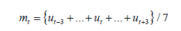
The following notation is used throughout the paper: Ut indicates the cumulative number of deaths on the t-th day; ut indicates the daily count of deaths on the t-th day. Since the reported data of daily counts typically fluctuate around the trend curves, we use the seven-day moving average:
Day t=1 is fixed at the date of the maximum daily number mt. The Gumbel cumulative distribution function is given as:
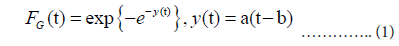
where a and b are the parameters that determine the shape (a) and position (b) of the distribution. Parameter b corresponds to the position of the peak. Using the relation ln FG(t)=−e−y(t), the probability density function for the Gumbel distribution fG(t) is given by:

In order to estimate Ut and mt, it is necessary to know the total number N , and:

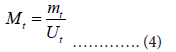
This method uses the value Mt defined as:
where Mt can be approximated by:
Thus, we have
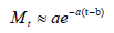
which can be obtained from the reported daily numbers.
The next task is to estimate the parameters of y(t)=a(t − b). Applying a logarithmic transformation, we de ne Lt as

Thus, Lt may be approximated by a linear function of t as:
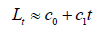
and coefficients c0 and c1 can be obtained using linear regression. From these values, we have estimates of the Gumbel parameters:

The regression analysis uses time window T having 12 elements:
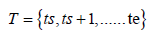
denoted as W[ts, te].
The final step is the estimation of the total number Ne. We use the average of the ratio:
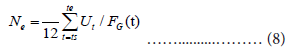
Then, the estimate of Ut is given by:
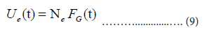
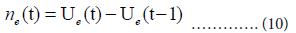
We use the cumulative number Ue(t) for our estimation of the daily number ne(t):
Results
Analysis for 8 countries in Europe and North America
Table 1 shows the time window for the regression analysis and the estimated Gumbel parameters. Column m shows the maximum daily number using the seven-day moving average mt; column me gives the maximum ne(t) calculated by Eq (10) (Table 1).
The Netherlands, Germany and Belgium
Figure 1A shows comparisons of the reported data for the Netherlands, Germany, and Belgium with the Gumbel model estimates. Day 1 is fixed at April 6 (the Netherlands), April 18 (Germany), and April 11 (Belgium) of 2020. Parameter estimation for the time course of the outbreak was conducted using two time windows for the regression analysis. The upper panels show the estimated daily numbers for the three countries for windows W(−11,0) and W(−19,−8). The lower panels show Lt for reported data and the estimated lines c0 + c1t for both time windows. As shown, the linear regression model provides a good fit for the data of the Netherlands, Germany, and Belgium. From Table 1, we note that the analysis of Belgium with two time windows provides very similar estimates of the model parameters (Figures 1A- 1F).
| Country | Window | m | me | Ne | a | b |
|---|---|---|---|---|---|---|
| Netherlands | W[-11, 0] | 154 | 146 | 4,870 | 0.08164 | 1.559 |
| W[-19, -8] | 0 | 164 | 6,601 | 0.06766 | 6.019 | |
| Germany | W[-11, 0] | 233 | 218 | 9,371 | 0.06334 | -1.392 |
| W[-19, -8] | 0 | 202 | 7,475 | 0.07355 | -4.612 | |
| Belgium | W[-11, 0] | 286 | 281 | 11,247 | 0.06795 | 1.782 |
| W[-19, -8] | 0 | 274 | 10,999 | 0.06785 | 1.596 | |
| Italy | W[-11, 0] | 822 | 789 | 30,850 | 0.0696 | 1.009 |
| W[-15, -4] | 0 | 936 | 46,123 | 0.05521 | 7.125 | |
| W[-19, -8] | 0 | 1189 | 65,859 | 0.0491 | 12.064 | |
| Sweden | W[-11, 0] | 99 | 95 | 3,882 | 0.06687 | 0.882 |
| W[-15, -4] | 0 | 129 | 7,100 | 0.04924 | 10.007 | |
| W[-19, -8] | 0 | 187 | 12,277 | 0.04139 | 18.473 | |
| United Kingdom | W[-11, 0] | 942 | 747 | 29,444 | 0.06897 | 5.321 |
| W[-15, -4] | 0 | 1048 | 53,037 | 0.05375 | 13.075 | |
| W[-19, -8] | 0 | 2441 | 1,58,757 | 0.0418 | 26.759 | |
| Canada | W[-11, 0] | 177 | 162 | 10,481 | 0.04208 | 2.066 |
| W[-15, -4] | 0 | 148 | 7,062 | 0.05719 | -5.88 | |
| W[-19, -8] | 0 | 145 | 6,198 | 0.06358 | -8.175 | |
| United States of America | W[-11, 0] | 2715 | 3064 | 1,73,991 | 0.04788 | 9.882 |
| W[-15, -4] | 0 | 2585 | 1,28,996 | 0.05488 | 5.37 | |
| W[-19, -8] | 0 | 2034 | 85,357 | 0.06482 | 0.042 |
Table 1: Parameters of the analysis for 8 countries in Europe and North America.

Figure 1: Gumbel model estimation based on time-series data of the Netherlands, Germany, and Belgium. Upper panels: Daily number of deaths for (A) The Netherlands; (B) Germany; (C) Belgium. The vertical axes in the panels show the daily numbers. Lower panels: Lt and the linear regression lines for (D) The Netherlands; (E) Germany; (F) Belgium.
Note: ( ) Reported data; (
 ) Theoretical estimates (W(-11, 0); ( ) (W(-19, -8)).
Italy, Sweden and the United Kingdom
Figures 2A-2F show comparisons of the reported data for Italy, Sweden, and the United Kingdom with the Gumbel model estimates. Day 1 is fixed at March 31 (Italy), April 14 (Sweden), and April 11 (the United Kingdom) of 2020. Parameter estimations are performed with three time windows. As shown in Table 1, the regression analysis with W(−11,0) and W(−15−4) provides good estimates of m and b; however, the analysis with W(−19,−8) fails in the estimation of these parameters. Figure 3A shows that the Gumbel model fits the daily numbers of the three countries reasonably well. Figure 3B indicates that the linear regression analysis using early-stage data does not follow the overall trends (Figures 2A-2F and 3A-3C).

Figure 2: Gumbel model estimation based on the time-series data for Italy, Sweden, and the United Kingdom. Upper panels: Daily number of deaths for (A) Italy; (B) Sweden; (C) United Kingdom. The vertical axes in the panels show the daily numbers. Lower panels: Lt and the linear regression lines for (D) Italy; (E) Sweden; (F) United Kingdom.
Note: ( ) Reported data; ( ) Theoretical estimates (W[-11, 0]); ( )(W(-15, -4)).

Figure 3: Gumbel model of the linear regression lines based on the data for (A) Italy; (B) Sweden; (C) the United Kingdom.
Note: (  )The results of the reported data; (
 ) The theoretical estimates using W(-19, -8).
Canada and the United States
The upper panels of Figure 4A show the daily numbers of deaths in Canada and the U.S. The lower panels give the results of the linear regression analysis. Day 1 for Canada is May 4; for the U.S., Day 1 is April 19. The reported data for Canada form an uneven curve with several bumps and estimates of parameter b with W(−15−4) and W(−19,−8) in Table 1 appear to indicate a small peak around t=−10. The reported curve for the U.S. also shows a large bump around the peak. The coefficients of determination R2 in the regression analysis are 0.842 for W(−11,0), 0.903 for W(−15,−4) and 0.983 for W(−19,−8). Thus, the windows at the early phase may give reliable estimates of the Gumbel parameters. In general, the Gumbel model ts the data at a reasonable level for both Canada and the U.S (Figures 4A-4D).

Figure 4: Gumbel model estimation of the daily number of deaths and the linear regression lines: (A) Daily numbers for Canada; (B) Daily numbers for the U.S.; (C) Regression lines for Canada; (D) Regression lines for the U.S.

England and 7 NHS regions
Table 2 shows the windows for the regression analyses and the estimated model parameters for England and its 7 NHS regions. To support our assumption of applying the Gumbel distribution, the table includes the results using window W(−7,4) for all of the NHS regions except London (Table 2).
| Country | Window | m | me | Ne | a | b |
|---|---|---|---|---|---|---|
| England | W[-11, 0] | 785 | 838 | 35,371 | 0.06439 | 5.27 |
| W[-15, -4] | 0 | 1,019 | 49,465 | 0.05601 | 9.695 | |
| W[-19, -8] | 0 | 1,931 | 1,21,106 | 0.04334 | 21.658 | |
| London | W[-11, 0] | 213 | 215 | 8,768 | 0.06666 | 4.056 |
| W[-15, -4] | 0 | 226 | 9,511 | 0.0646 | 5.02 | |
| W[-19, -8] | 0 | 356 | 18,823 | 0.05137 | 13.568 | |
| East | W[-7, 4] | 90.7 | 83.9 | 2,901 | 0.07863 | 0.312 |
| W[-11, 0] | 0 | 86.3 | 3,197 | 0.07342 | 1.571 | |
| W[-15, -4] | 0 | 90.3 | 3,568 | 0.06884 | 2.988 | |
| South West | W[-7, 4] | 37.9 | 35.2 | 1,279 | 0.07478 | 2.825 |
| W[-11, 0] | 0 | 43.9 | 2,086 | 0.05724 | 9.565 | |
| W[-15, -4] | 0 | 50.6 | 2,609 | 0.05277 | 12.577 | |
| South East | W[-7, 4] | 91.3 | 86.6 | 3,424 | 0.06879 | 2.387 |
| W[-11, 0] | 0 | 96.5 | 4,510 | 0.05814 | 6.456 | |
| W[-15, -4] | 0 | 112.7 | 5,995 | 0.0511 | 10.742 | |
| Midlands | W[-7, 4] | 147.3 | 132.6 | 4,238 | 0.08422 | 0.604 |
| W[-11, 0] | 0 | 153.2 | 5,954 | 0.07001 | 3.975 | |
| W[-15, -4] | 0 | 262.8 | 14,300 | 0.04997 | 15.336 | |
| North West | W[-7, 4] | 127.6 | 122.7 | 4,617 | 0.07224 | 3.339 |
| W[-11, 0] | 0 | 127.8 | 5,151 | 0.06746 | 4.83 | |
| W[-15, -4] | 0 | 369.4 | 25,761 | 0.03898 | 27.639 | |
| North East | W[-7, 4] | 104.3 | 97.8 | 2,935 | 0.09062 | 2.831 |
| W[-11, 0] | 0 | 113.6 | 4,109 | 0.07519 | 6.601 | |
| W[-15, -4] | 0 | 861 | 60,591 | 0.03863 | 37.245 |
Table 2: Parameters of the analysis for England and its 7 NHS regions.
England and London: The population of London is approximately 15% of England’s total. London has the highest population density among the 7 NHS regions. Day 1 for Eng- land is April 8; for London, Day 1 is April 6. Figure 5A shows the results of the estimation of the daily numbers and the linear regression lines for England and London. For England, the Gumbel model explains well the reported data with W(−11,0). However tting with W(−15,−4) overestimates the data. For London, the model gives similar results with W(−11, 4) and W(−15−4). Figure 5A shows poor results with W(−19,−8) for England and London. Table 2 also shows exceedingly large values of me and b estimated with this W(−19,−8) window (Figures 5A-5D and Figures 6A and 6B).

Figure 5: Gumbel model estimation of the daily number of deaths and the linear regression lines: (A) daily numbers for England, (B) daily numbers for London, (C) regression lines for England, and (D) regression lines for London.
 The vertical axes in the upper panels show the daily numbers.

Figure 6: Gumbel model estimation of linear regression lines based on the data of (A) England; (B) London with W[−19, −8].
 Theoretical results.
East, South West and South East: Table 2 shows the results for the East, South West, and South East regions. Dates of the peak are April 10 for East, April 8 for South West, and April 9 for South East. East and South East are neighbors of London. Figure 7A shows the results of the analysis for the East, South West, and South East regions. The estimation with W(−7, 4) fits the time-series data of the three regions satisfactorily. The data for the East region are also well represented with W(−11, 0) and W(−15,−4). On the other hand, the analysis with these windows overestimates the daily numbers for the South West and South East regions (Figures 7A-7F).

Figure 7: Upper panels: Estimation of the daily number of deaths based on the data for (A) East, (B) South West, and (C) South East. The lower panels show the results of the linear regression analysis for the corresponding regions: (D) East, (E) South West, and (F) South East.


Midlands, North West and North East NHS areas: The central and northern part of England consists of the Midlands, North West, and North East regions. The dates of the maximum daily number are April 7 for the Midlands, April 10 for North West, and April 7 for North East. Table 2 shows that the linear regression analysis with W[−7,4] and W(−11,0) gives reasonable estimates of the peak height and position for these regions. However the analysis with W(−15,−4) fails to estimate the peak properties of the three regions. Figures 8A-8F reports the results with W(−7,4) and W(−11,0). The linear regres- sion analysis for both windows satisfactorily reproduces the daily numbers of deaths. Figure 9A shows the regression lines with W(−15,−4). This gure sug- gests that the regression analysis using early-stage data can sometimes fail to reproduce local level time-series data (Figures 8A-8F and 9A- 9C).

Figure 8: Upper panels: Estimation of the daily number of deaths based on the data for (A) Midlands, (B) North West, and (C) North East. The vertical axes show the daily numbers. The lower panels show the results of the linear regression analysis for the corresponding regions: (D) Midlands, (E) North West, and (F) North East.


Figure 9: Results of the linear regression analysis with Window (-15, -4) based on the data for (A) Midlands; (B) North West; (C) North East.


Discussion
This section presents two extensions of our approach: (1) the hazard function or intensity function given in [4] for mortality analysis, and (2) piecewise regression analysis for change point detection.
The hazard function μ(t) is de ned as:
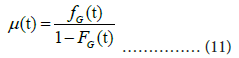
Although the hazard function need not be monotonic, the function of the Gumbel distribution is monotonically increasing. The upper bound of μ(t) is the shape parameter a. The estimates of FG(t) and fG(t) for the reported data are:
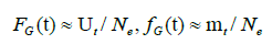
where the estimate of total number Ne=9371 is listed in Table 1. Panel (A) of Figure 10A shows the theoretical hazard function and that estimated from the reported data. The theoretical upper bound is a=0.06334, as listed in Table 1, the upper bound of the estimated function is ~0.05 (Figures 10A and 10B).

Figure 10: Panel (A) The hazard function for Germany with the parameters of Window (-11, -0) in Table 1. Black points are the estimated hazard function using the reported data. The theoretical estimates are indicated by the solid red line. The blue dotted line shows the theoretical upper bound of µ(t); Panel (B) The piecewise regression analysis for Sweden.
 regression.
Our piecewise regression analysis was conducted in the statistical environment R, with the package \segmented” downloaded and applied for the calculation. The reported data for Sweden are used to illustrate. We coded the R program using the prototype in (www.statology.org/ piecewise-regression-in-r). The right panel of Figure 10A shows the results of the regression; see Panels (B) and (E) in Figure 2A for a comparison. The input data were Lt (−24 ≤ t ≤ 49) and an initial value for breakpoint t=9. The segmented() function detected a breakpoint at t=15 ± 3.68. The two resulting linear regression lines are:
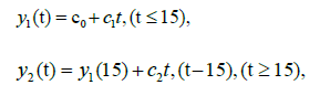
where c0=2.6907, c1=0.05393, and c2=0.03997. The coefficient of determination here is R2=0.989. Wieland reported a detailed breakpoint study investigating the effectiveness of interventions in Germany [15].
Conclusion
A mathematical model that effectively captures the characteristics of virus spread is a key tool for science-based public health management. In this study, we applied the Gumbel distribution function of EVT to analyze time-series data on rst-wave COVID-19 deaths in 8 countries, as well as England’s 7 NHS regions. The proposed method makes use of the Gumbel distribution to model the daily number of deaths. The distribution has three parameters in need of estimation: total number Ne, shape parameter a, and position parameter b. Parameter Ne can be removed from the estimation process by taking the ratio Mt of the seven-day moving average mt to Ut as given in Eq. (4). The next step is to perform logarithmic transformation Lt according to Eq. (6), which enables us to estimate parameters a and b using basic linear regression analysis. Selecting 8 countries and 8 regions, we estimated the time to the peak and the height of the peak for each area. The proposed method assumes that future data can be estimated by extrapolating an appropriate linear function. Special attention is thus given to the relative positions from the peak for the time window of the regression analysis. Although, in general, the Gumbel model was shown to describe the time-series data of COVID-19 deaths rather well indicate a lack of t in several areas for time windows in the early stages. The reported data deviate significantly from the linear trend. As part of our ongoing work, we are now seeking to develop an alternative approach for estimating model parameters.
Data Availability
The datasets generated and analyzed during the current study are available from the corresponding author upon reasonable request.
Author Contributions
The present study was conducted equally by the authors.
Competing Interests
The authors declare no competing interests.
References
- Kermack WO, McKendrick AG (1927) A contribution to the mathematical theory of epidemics. Proc Roy Soc London A 115: 700-721.
[Crossref] [Google Scholar] [PubMed]
- Brauer F (2008) Compartmental models in epidemiology. In: Mathematical Epidemiology, Lecture Notes in Mathematics. Basel: Springer Nature, Switzerland 1945: 19-79.
- Zou Y, Pan S, Zhao P, Han L, Wang X, et al. (2020) Outbreak analysis with a logistic growth model shows COVID-19 suppression dynamics in China. PLoS ONE 15: e0235247.
[Crossref] [Google Scholar] [PubMed]
- Gumbel EJ (1958) Statistics of extremes. New York: Columbia University Press, United States.
[Crossref]
- Coles S (2001) An Introduction to statistical modeling of extreme values. (2001st edn). London: Springer-Verlag, United Kingdom.
- Wong F, Collins JJ (2020) Evidence that coronavirus superspreading is fat-tailed. PNAS 117: 29416-29418.
- Fisher RA, Tippett LHC (1928) Limiting forms of the frequency distribution of the largest or smallest member of a sample. Proc Cambridge Phil Soc 24: 180-190.
- Ohnishi A, Namekawa Y, Fukui T (2020) Universality in COVID-19 spread in view of the Gompertz function. Prog Theor Exp Phys 2020: 123J01.
- Gompertz (1825) On the nature of the function expressive of the law of human mortality, and on a new mode of determining the value of life contingencies. Phil Trans R Soc 115: 513-585.
- Berger RD (1981) Comparison of the Gompertz and logistic equations to describe disease progress. Phytopathology 71: 716-719.
- Fleming RA (1983) Development of a simple mechanistic model of cereal rust progress. Phytopathology 73: 308-312.
- Furutani H, Hiroyasu T (2022) Estimation of COVID-19 cases in Japanese prefectures using a Gumbel distribution. Arch Clin Biomed Res 6: 756-764.
- Furutani H, Hiroyasu T (2023) Analysis of the sixth wave COVID-19 outbreak in Japan. Proc ISAROB 2023: 1-5.
- Furutani H, Hiroyasu T, Okuhara Y (2022) Method for estimating time series data of COVID-19 deaths using a Gumbel model. Arch Clin Biomed Res 6: 50-64.
- Wieland T (2020) A phenomenological approach to assessing the effectiveness of COVID-19 related nonpharmaceutical interventions in Germany. Saf Sci 131: 104924.
[Crossref] [Google Scholar] [PubMed]
Citation: Furutani H, Hiroyasu T (2023) Linear Regression Analysis of COVID-19 Time-Series Data using the Gumbel Distribution. J Infect Dis Ther 11:553 DOI: 10.4172/2332-0877.1000553
Copyright: © 2023 Furutani H, et al. This is an open-access article distributed under the terms of the Creative Commons Attribution License, which permits unrestricted use, distribution, and reproduction in any medium, provided the original author and source are credited.
Select your language of interest to view the total content in your interested language
Share This Article
Recommended Journals
Open Access Journals
Article Tools
Article Usage
- Total views: 1990
- [From(publication date): 0-2023 - Dec 01, 2025]
- Breakdown by view type
- HTML page views: 1609
- PDF downloads: 381