Research Article Open Access
Households Income Poverty and Inequalities in Tanzania: Analysis of Empirical Evidence of Methodological Challenges
Lusambo LP*Department of Forest Economics, Sokoine University of Agriculture, Morogoro, Tanzania
- Corresponding Author:
- Lusambo LP
Department of Forest Economics
Faculty of Forestry and Nature Conservation
Sokoine University of Agriculture
Morogoro, Tanzania
Tel: +255 23 260 3511
E-mail: lusambo_2000@yahoo.com
Received September 08, 2015; Accepted April 18, 2016; Published April 29, 2016
Citation: Lusambo LP (2016) Households’ Income Poverty and Inequalities in Tanzania: Analysis of Empirical Evidence of Methodological Challenges. J Ecosys Ecograph 6:183. doi:10.4172/2157-7625.1000183
Copyright: ©2016 Lusambo LP. This is an open-access article distributed under the terms of the Creative Commons Attribution License, which permits unrestricted use, distribution, and reproduction in any medium, provided the original author and source are credited.
Visit for more related articles at Journal of Ecosystem & Ecography
Abstract
The overarching objective of this study was to assess poverty situation in Tanzania using a multitude of approach so as to provide empirical evidence of conceptual and methodological challenges encountered in poverty analysis studies. Specifically, the study strove to: (1) analyse the poverty situation in the study sites, (2) assess income inequality in study sites, and (3) determine the method that could be commonly employed to measure poverty , with a view to improve consistency in poverty statistics. A sample of 568 respondent households was involved in the study. Data was collected through household questionnaire, key informant interview, focus group discussion and researcher’s direct observations. Collected data was analysed using statistical package for social sciences (SPSS) and Microsoft excel computer programmes. Different poverty lines have provided different results regarding the number of households which are poor. Relative poverty line of 40% of the median income gave the lowest value of poverty in the study area, while the ethical poverty line provided the highest rate of poverty. Accordingly, it was found that using selected poverty lines: overall, 29.3% - 98.2% of households are poor. In rural areas, 24.5% - 96.8% of households are poor. In peri-urban areas, it was found that 20% to 100% (depending on the poverty line used) were poor, while in urban areas the poverty rate was found to be between 37.1% to 99%. Using weighted geometric mean of relative and absolute poverty lines (ρ = 0.7) at relative poverty line of 50% of median income and absolute poverty line of US$ 1-a-day (2005PPP): Overall, 53.5% of households are poor, and poverty rates in rural, peri-urban and urban areas are 55%, 53% and 46% respectively. The findings revealed further that the poverty gap ratio and severity ratio are highest in urban areas (0.35 and 0.29 respectively), medium in rural area (0.33 and 0.24 respectively) and minimum in peri-urban area (0.29 and 0.20 respectively). Household income inequality in the study area is high (Gini Coefficient = 0.773), with variations in the strata as follows: rural areas (Gini Coefficient = 0.821); peri-urban areas (Gini Coefficient = 0.574); and urban areas (Gini Coefficient = 0.717). Inter-strata inequality index in the study area (depending on the method used) ranged between 0.158 – 0.172, while inter-regional inequality index ranged between 0.004 and 0.116. Some recommendations have been put forward: Firstly, in the determination of poverty rates (head counts) the appropriate yardstick to be used is weighted geometric mean of relative and absolute poverty lines (ρ = 0.7) at relative poverty line of 50% of median income and absolute poverty line of US$ 1-a-day (2005PPP). Secondly, in the determination of household income inequality, Gini Coefficient should be used. Thirdly, the Hoover coefficient (Robin Hood Index) is a more appropriate metric for regional and inter-strata inequality.
Keywords
Poverty; Inequality; Household income
Introduction
An overview of poverty concept
Reducing poverty and inequality is a cornerstone of development policy of any nation [1]. Poverty definitions and measurements have important ramifications for targeting its reduction strategies [2]. While there is a widespread agreement on the desirability of poverty reduction, defining poverty is more controversial. There is no objectively correct definition of poverty, and most commentators accept that any definition must be understood in relation to a specific political, economic and social context [3]. Empirical evidence suggest that poverty rates vary a lot when different concepts and measures are used, thus clearer definitions and measures are essential for poverty-centred development policies [2]. Poverty can be conceptualised and measured in different ways. The conventional economic approach focuses on the quantifiable poverty lines based solely on consumption and expenditure patterns. While the poverty line is an important measure of poverty in a country over time, poverty goes beyond income level: it includes lack of access to health and education, respect, isolation from the community, and a feeling of powerlessness and hopelessness. Poverty is actually multi-dimensional, and many of its dimensions are often hidden. People whose main source of income is their farm, are five-times more likely to be poor than their counterparts who receive a wage from the public or private sector [4]. Handley et al. [5] posited that poverty is not an easy concept to define, as a result a range of definitions exist, influenced by different disciplinary approaches and ideologies. Madulu [6] reported that a poor person is a one whose standard of living falls below the minimum acceptable level (poverty line), and can be absolute or relative. Poverty is a multidimensional phenomenon, and can be defined using three different concepts: income, basic needs, and capability. Of these, the most commonly used concept is income, where a person is poor if her/ his income is below a certain amount. The basic need concept considers material requirements for a minimally fulfilling life. These are normally understood to include factors such as basic health care and education. The capability perspective concentrates on factors such as adequate nutrition, clothing and shelter, but also considers social aspects such as partaking in the life of the community [3,5].
There are many definitions, as well as intense debate, about the poverty situation. As a matter of definition, it is imperative to distinguish four types (degrees) of poverty: extreme or absolute poverty, moderate poverty, relative poverty [7] and subjective poverty [8]. Absolute poverty means that households cannot meet basic needs for survival. They are chronically hungry, unable to access health care, lack amenities of safe drinking water and sanitation, cannot afford education for some or all children, and perhaps lack rudimentary shelter [7,9,10]. Relative poverty depends on the social context, and may be objectively assessed or subjectively measured [11]. Blackorby and Donaldson [12] reported that relative poverty is something whose value is unchanged when all incomes and the poverty line itself are multiplied by a positive scalar, while the absolute poverty index is one whose value depends on the income of the poor. Subjective poverty, Duclos and Araar [8] refers to poverty as perceived by the households themselves. Generally speaking poverty may be socially or economically/statistically defined (Figure 1). Saunders et al. [13] make the distinction between absolute poverty and overall poverty: absolute poverty is a “condition characterised by severe deprivation of basic human needs including food, safe drinking water, sanitation facilities, health, shelter, education and information − it depends not only on income but also on access to services. Overall poverty is a wider concept including not only lack of basics, but also lack of participation in decision making, and in civil, social and cultural life. Arnold [14] for instance reported that poverty has generally been defined as insufficient food, income, and inputs to maintain adequate standard of living, with the latter sometimes being defined to include quality of life.
Ortiz et al. [15] posited that the consequences of poverty and inequality are very significant for children. Children experience poverty differently from adults; they have specific and different needs. While the adults may follow into poverty temporarily, falling in poverty in childhood can last a life-time: rarely does a child get a second chance at an education or healthy start life. Poverty as a public policy concern, whether at the global, national or community level, is now widely considered to be a multidimensional problem. Over the last few decades, new perspectives on poverty have challenged the focus on income and consumption as the defining condition of poor people. Studies of the problems of poor people and communities, and of the obstacles and opportunities to improving their situation, have led to an understanding of poverty as a complex set of deprivations [2].
Poverty measurements
Poverty lines or thresholds are another contentious area in poverty analysis. Duclos and Araar [8] reported that there are three major issues to be addressed in the estimation and use of poverty lines. First, the space in which well-being is to be measured should be lucidly defined: utility, income, “basic needs”, functioning or capabilities. Second, it must be determined whether the interest is in absolute- or in relative-poverty line terms. Third, it must be chosen whether it is by someone’s capacity to function or by someone’s actual functioning that a poor person is judged. Absolute poverty lines can be interpreted as fixed in any one of the spaces in which we wish to assess well-being. Conversely, a relative poverty line would depend on the distribution of well-being (including the utilities, living standards, functioning or capabilities). Considerable controversy exists on whether absoluteness or relativity is the better property for a poverty threshold. Saunders et al. [13] argue that income and expenditure measures are commonly used to establish poverty lines representing respectively, the availability of cash resources and the standard of living approaches to measuring the extent and composition of poverty. The authors assert that there is little overlap between income and expenditure poverty and that very few households are both income- and expenditure-poor.

Figure 1: Understanding the poverty concept.
When poverty is defined in absolute terms, the World Bank and the United Nations Millennium Development Movement defines poverty using an income threshold (at a purchasing power parity) of US$ 1 a day per person for Africa; US$ 2 a day per person for Latin America; and US$ 3 a day per person for Central and Eastern Europe [16,17]. People living below US$ 1-a-day at purchasing power parity (PPP) are considered to be under extreme poverty, whereas those living between US$ 1 and US$ 2 a day per person are said to be under moderate poverty [7,18-22]. Literature suggests that there are three purchasing power parity (PPP) base years recognised by the World Bank, and that the decision on which base year to use when defining the poor remains subjective.
The World Bank’s poverty line of US$ 1-a-day per person at purchasing power parity is equivalent to: US$ 31-a-month per person PPP 1985 (US$ 1-a-day per person), US$ 32.74-a-month per person PPP 1993 (US$ 1.08-a-day per person) [23,24], and US$ 1.25-a-day per person PPP 2005 [24]. Pogge [23] reported that the relevant equivalency of a Word Bank US$ 1-a-day poverty line was US$ 31-a-month per person in 1999 and is US$ 49-a-month per person in 2008. Edward [25] has strongly criticised the World Bank’s dollar-a-day per person (at purchasing power parity) in that it is poorly defined and variable between countries: it disguises the current scale of absolute poverty and understates the challenges that eliminating absolute poverty poses for the developed world. Lusambo proposes what is called the ethical poverty line to be US$ 2,200 per person per year (at purchasing power parity). OECD [3] posits that there are two types of ethical poverty lines, namely: minimum ethical poverty line (US$ 1.9 -a-day) and global ethical poverty line (US$ 2.7-a-day).
United States and the United Kingdom, in contrast, use absolute poverty line measures to separate the poor from the non-poor. In the UK for example a person living below US$ 14.4 a day is considered poor [26]. In the United States, for year 2007, a person aged 65 or above was considered poor if he/she had an annual income below US$ 9,944; while a person less than 65 years was considered to be poor if he/she had an annual income below US$ 10 [27]. Long [28] reported that the relative poverty line is usually taken as a percentage of the mean or median income. It is commonly set at half of the mean or median household income. The choice of the percentage cut-off is arbitrary, as it will not necessarily represent the actual dividing line between those with low income and the rest. Households with income below the relative poverty line are not necessarily poor, but they are in the lower-income group compared with the population at large. As a result, several cut-offs are sometimes employed. For example, relative poverty lines could be set at 40%, 50% and 60% of the mean or median income. There are no fixed guidelines regarding the use of mean or median income to set the relative poverty line. The advantage of using mean income as a cut-off lies in the ease of interpretation. Relative poverty lines used for instance by OECD and European Union countries are based on “economic distance”, a level of income set at 40%, 50% or 60% of the median household income. The European Union in particular has decided to use 60% of the median income as the relative poverty line below which a person or household is considered poor [10,16,29].
When it comes to choosing between median or mean income as the basis for an explicit relative poverty line, the majority of researchers prefer the median for two main reasons: first, when the median is used, the reference point is a person, family or household who is at the middle of the distribution, with half above and half below them. When mean is used, there may be no one involved at all, as there may be no person, family, or household who has this exact income. Second, the median, unlike the mean, is less affected by the extreme values of the income distribution and by sampling fluctuations, thus is a less sensitive measure of central tendency of income distribution [13,28,30]. Madden [31] explained that many people view absolute poverty line as unreasonable since (almost always) it doesn’t accordingly change with time.
Madden [31] and Foster [32] pointed out that the weighted geometric average of the relative and absolute thresholds may be used. This poverty line can be presented algebraically using equation 1.
where: 0 <ρ <1
Z is weighted geometric average of poverty lines
Zr is relative poverty line
Za is absolute poverty line
ρ is income elasticity of the poverty line
This form of poverty line has a property that one percent increase in central measure leads to a ρ percent increase in poverty line. A value of ρ equal to zero implies an absolute poverty line while a value of ρ equal to one implies a purely relative poverty line. The absolute/relative poverty line debates now become a question of “how relative?” with ρ the relevant decision variable. Madden [31] posits that the upper bound of ρ = 0.70.
Subjective poverty lines on the other hand can be established using subjective information on the link between living standards and well-being. One source of information comes from interviews on what is perceived to be a sound poverty line, using question such as [8]: “We would like to know which net family income would, in your circumstance, be the absolute minimum for you. That is to say, that you would not be able to make both ends meet if you earned less”. The answers are subsequently regressed on the incomes of the respondents. The subjective poverty line is given by the point at which the predicted answer to the minimum income answer equals the income of respondents. An alternative approach to estimating subjective poverty line is to ask respondents whether they feel that their incomes are below the poverty line, without directly asking what the value of poverty line should be. Answers are coded 0 or 1 depending on whether the respondents feel that they are poor or not alongside the respondents’ income. The estimate of the poverty line is that which best reconciles the distribution of those answers with that of the respondents’ incomes.
Incidence of poverty, depth of poverty, and severity of poverty
Many people (e.g. Long [28]; Madden [31]; Simler and Arndt [33]; Foster [32]; Saunders et al. [13]; Delamonica and Minujin [34]; Son and Kakwani [35]) have reported that poverty measurements and analysis should strive to capture: incidence of poverty − how many people are poor?; depth of poverty − what is the extent or depth of poverty (poverty gap ratio)?; and severity of poverty − how severe is the extent of poverty? To answer these questions, the authors have suggested the use of equation 2.
Where Yi is the income of the ith person, q is the number of people with income below poverty line, Z is the poverty line, and n is the total number of people. The author further decomposes this generic equation into equations for head count index, poverty gap ratio, and Foster-Greer-Thorbeke P2 measure.
(a) Head Count Index (α=0): The head count index (H), which is the indicator that measures the incidence of poverty gives the proportion of persons whose income are below the poverty line. Its computational equation is equation 3.
(b) Poverty gap ratio (α=1): The poverty gap (PG) ratio is used to gauge the depth of poverty. It is based on the aggregate poverty deficit of the poor relative to the poverty line. Essentially, the poverty gap ratio is the average proportionate poverty gap across the all persons (with zero gap for the non-poor persons). Its computation is effected through the use of the equation 4.
The poverty gap can also be computed from the equation 5 [31,36,37].
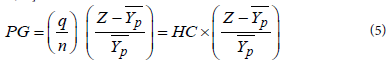
The variables in these equations are as follows:
q is the number of people below the poverty line
n is the total number of people in the society
z is the poverty line income
 is the average income of those people below the poverty line; and HC is the head count ratio of people under poverty line.
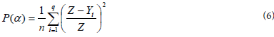
(c) Foster-Greer-Thorbeke measure (α=2): Long [28] has hinted that it is not easy to interpret this index. It is the measure of severity of poverty whereby the poverty of the poor are weighted by those poverty gaps in assessing the aggregate poverty, with more weight given to the poorest among the poor. Its computational formula is: equation 6.
Delamonica and Minujin [34] suggested that in any society, there is a continuum of deprivation.
Income inequality: an overview
A wide number of inequality measures are available in literature. The most commonly and widely used inequality metric is the Gini coefficient (also called Gini index) [38-41]. This measure is typically defined in terms of the Lorenz curve which is essentially a cumulative frequency plot (Figure 2). This metric can be defined graphically as the ratio of the area between the line of perfect equality and the Lorenz curve, and the total area below the line of perfect equality. The Gini coefficient can also be computed mathematically. Different forms of computational formulae are available from different literature. According Marsh and Schilling [40], Dixon et al. [42], and Damgaard and Weiner [43], the Gini coefficient (G) is most easily calculated from unordered size data as the “relative mean difference”, i.e., the mean of the difference between every possible pair of individuals, divided by the mean size (equation 7).
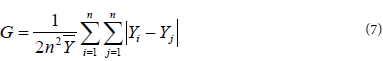
Variables are as follows: Yi and Yj are per-capita development parameters (e.g. per-capita income) observed respectively in region/ individual i and region/individual j, n is the overall number of regions, and  is the average income of the regions.
Alternatively, if the data are ordered by increasing number of individuals, then, the Gini Coefficient (G) is computed using equation 8 [43-45].
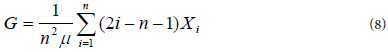
where i=1, …, n individuals or equal-sized groups in order of increasing income, Xi; and μ is mean equal income. The value of G ranges between 0 and 1. A value of zero indicates perfect inequality (everyone has the same income). A value of one indicates perfect inequality (one person has all the income).
Habibov and Fan [46] and World Bank [47] presented that in measuring inequality, Gini Coefficient is one of the most commonly used measure, and that using Gini Coefficient has advantage insofar as it satisfies three important principles, which are. Anonymity: it does not take into account who the wealthy and poor are. Scale Independence: it does not take into account the size of the economy, wealth of the country, and the size of population in the country. Transfer Principle: if income is transferred from the wealthy to the poor, the Gini Coefficient demonstrates more income distribution. As a rule of thumb, the Gini Coefficient is expressed in the percentage form as Gini Index that is equal to Gini Coefficient multiplied by 100. Habibov and Fan [46] pointed out disadvantages of using Gini Coefficient: it is highly sensitive to selection of unit of analysis (e.g. individuals or households), grouping (e.g. deciles or quantile), and welfare indicators (e.g. income or consumption), and that it is more common to calculate Gini of income.

Figure 2:Conceptual Lorenz curve
Despite these limitations, the Gini coefficient has been used extensively in the public health literature, and it remains the most popular measure of income inequality. Yet because it is highly sensitive to inequalities in the middle of the income spectrum, the Gini coefficient is not “neutral” or value free. Because of this property, the Gini coefficient is best seen as simply one of the many strategies available for the operationalisation of income inequality [48]. The author (ibid) highlights other measures of income inequality as follows: Atkinson index, Coefficient of variation (CV), Decile ratios, Generalised entropy (GE) index, Kakwani Progressivity index, and Sen Poverty measure. Another inequality metric is Hoover coefficient, also called Robin Hood [39-41,44]. Burkey [44] defines the Robin Hood Index as the proportion of income that must be reallocated from above-average earners to below-average earners to achieve an equal income distribution. It is also based on a Lorenz curve (Figure 2). It’s mathematical computational for Hoover coefficient (HC) is equation 9.
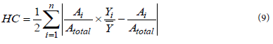
Definitions of variables used are as follows: Ai is the number of individuals in regions i, (regional populations), Atotal is the total population; Yi is the per capita development parameter observed in region i, and is the national average development parameter in the area (e.g. per capita national income); n is overall number of regions.
Theil index (T) is another commonly used measure of inequality [40,41,49,50]. Goodchild and Janelle [49] and Rey and Janikas [50], posited that Theil index is popularly used in regional inequality analyses, and is computed using equation 10.
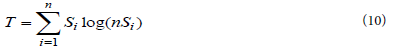
Where n is the number of regions, Yi is per-capita income in region i, and Si is expressed using equation 11.
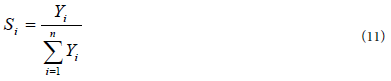
The T is bounded on the interval [0, log (n)], with 0 reflecting perfect equality (i.e. Yi = Yj ∀i, j) and the value of log (n) , which occurs when all income is concentrated in one region. The T measures systematic or global inequality of incomes across the regions at one point in time. Other alternative mathematical formulae for computing the same inequality metric (T) have been provided by Marsh and Schilling [40] (equation 12).
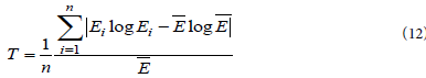
Variables are defined as follows: Ei and  are respectively, percapita income in region i and average per-capita income in all regions combined together, and n is the number of regions. Portvon and Felsenstein [41] suggested that Theil coefficient be computed using equation 13.
Where Yi and are respectively, per-capita income in region i and average per-capita income in all regions combined together, and n is the number of regions. On the other hands, Gibson et al. [51] and Bakar [52] has suggested that this inequality metric should be computed using equation 14.
where n is the number of people/groups, Yi is the per-capita income, and is the mean per-capita income for the whole area. Other measures of inequality which, albeit not used in the present study, are worth mentioning include [31,41,48] coefficient of variation (CV), Williamson index (WI), Atkinson index (AT), Coulter coefficient (CC), Decile ratio, Kakwani progressivity index; and Sen Poverty measure. All the equations highlighted above (i.e, equation 1 to equation 14) are presented in Table 1.
Problem statement and objectives of the study
The detailed review of pertinent literature on poverty and inequality has revealed that there exist considerable methodological challenges. There is no a single unanimously and objectively agreed upon definition of the term “poverty”. It is imperative that all people should have the same meaning of the phenomenon. As it stands now, efforts to reduce poverty (nationally, regionally and globally) are likely to fail, since different people have different concentration depending on the adopted definition(s) of poverty. Equally challenging (as evidenced by literature review) is the issue of objectively agreed-upon yardstick with which to measure the poor people. This is commonly known as “poverty lines”. There is a myriad of poverty lines which consequently makes it difficult to have reliable estimates of the extent of poverty. Two or more experts assigned to measure poverty in a given community are likely to have different results if they employ different poverty lines (yardsticks). The same scenario is experienced with regards to measurements of inequality.
Therefore, the overarching objective of this study was to assess poverty situation in Tanzania using a multitude of approach so as to provide empirical evidence of conceptual and methodological challenges encountered in poverty analysis studies. Specifically, the study strove to: (1) analyse the poverty situation in the study sites, (2) assess income inequality in study sites, and (3) determine the method that could be commonly employed to measure poverty , with a view to improve consistency in poverty statistics.
Methodologies
Study sites
This study was conducted with households in Morogoro and Songea districts (in Morogoro and Ruvuma regions respectively). Each District was sub-divided into three strata namely rural, peri-urban and urban areas; and sample households were drawn from each stratum. It sounds unreasonable to select the study area for research using a random sampling technique; one should make use of the available information that might quite logically guide the [53]. Selection of Morogoro and Ruvuma as study regions was guided by Carissa et al. [54] who carried out a deskwork study (based on an extensive literature review) to identify the regions within the country where critical ecosystem services for human well-being are stressed (proxy of poverty situation), signalling the need for immediate attention. The ecosystems functions covered were biodiversity, energy resources, water, and food and fibre production. It was envisaged that the findings of the study would inform and guide the selection of potential areas where a more detailed local-scale integrated assessment of the links between ecosystem services and human well-being can be carried out. The study established that Morogoro is a priority Region for ecosystems-related researches, because it is stressed in all the four ecosystem services. It also established that Ruvuma Region has serious data gaps in all the above-mentioned ecosystem services. The present study therefore considered these two regions as research-priority areas for povertyrelated studies.
| S/N | Equation | Reference |
|---|---|---|
| 1 |  |
Madden[31]; Foster [32] |
| 2 |  |
Long[28]; Madden[31]; Simler and Arndt [33]; Foster[32]; Saunders et al.,[13]; Delamonica and Minujin, [34]; Sonand Kakwani[35] |
| 3 |  |
|
| 4 | 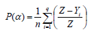 |
|
| 5 | 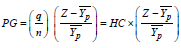 |
Werling[36]; Quah[37]; Madden [31] |
| 6 | 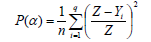 |
Long [28] |
| 7 | 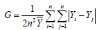 |
Marsh and Schilling [40],Dixon et al.,[42],Damgaard and Weiner [43] |
| 8 |  |
Burkey [44]; Dixon et al.,[42]; Damgaard and Weiner [43] |
| 9 | 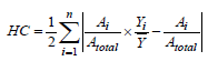 |
Bideleux and Lunden[39];Marsh and Schilling[40];Portvon and Felsenstein[41]; Burkey[44] |
| 10 | 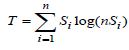 |
Goodchild[49];Rey and Janikas[50] |
| 11 |  |
|
| 12 | 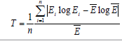 |
Marsh and Schilling [40] |
| 13 | 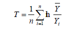 |
Portvon and Felsenstein[41] |
| 14 | 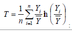 |
Gibson et al., [51] and Bakar[52] |
Table 1: Summary of selected equations for poverty measurements.
Study design
The design of the present study is a descriptive cross-sectional survey. It is a descriptive study because it sets out to rigorously describe household poverty situation in selected parts of Tanzania. It is a one-time cross-sectional study; it cannot therefore gauge the temporal variations or trends in the data collected. The sample design for the present study entailed nine steps: defining target population, defining sample frame, determining primary sampling units, defining secondary sampling units, defining reporting domain, defining explicit strata, defining measure of size, defining ultimate sampling units, and allocation of sample. The overall objective was to have a study sample which is sufficient and representative of the target population. The target populations for this study were households in Morogoro and Songea districts. The sampling frame was in three types depending on the sampling phase. During sampling of villages in rural areas and wards in peri-urban and urban areas, the sampling frame was the list of villages and list of wards in the municipalities respectively. During sampling of hamlets in rural areas and streets in peri-urban and urban areas, the sampling frame was the list of all hamlets in the selected villages and list of all streets in the selected wards respectively. When sampling households for the study, the sampling frames that were used are the updated lists of households registers in the sampled hamlets and streets. All chairpersons and executive officers in the selected study sites were asked to update lists of households in their respective areas by excluding households which no longer existed and/or adding those ones which were missing in their lists.
Stratified random sampling design was used in the present study. Stratification was carried out at two levels: (a) stratification of study sites in the study districts into rural, peri-urban and urban areas, and (b) stratification of respondents into wealth categories: low, medium and high. Figure 3 presents the approach used by the present study to stratify the study sites into rural, peri-urban and urban. Rural areas in the context of the present study refer to communities bordering the forests. Urban areas refer to the community residing fairly in the centre of municipality. Peri-urban areas refer to the areas geographically located within the municipality, but lying on its periphery.
Rural area sample selection: The first step was to get the list of all forests in each district, from respective District Forest Catchment Offices. Villages bordering the selected forests were operationally designated as rural areas. Out of villages bordering a selected forest, one village was randomly selected. Hamlet(s) were then randomly selected from each selected village. With the aid of village governments (through FGD), households in the selected hamlets were stratified into low-income, medium income and high-income. Finally, respondent households were randomly selected from each stratum using a random number table. Random selection of woodlands (forests), villages, and hamlets was made possible through the use of the playing cards method: the names of forests; villages or hamlets were written on the lower parts of the cards, the cards were then thoroughly mixed together, and the desired sample size randomly selected from the pool of the cards.
Urban area sample selection: The municipalities in each district were operationally designated as urban areas. The list of all wards in the municipality (urban area) was sought. The wards which are within the municipality, but are located on the periphery (i.e., bordering the municipality), were excluded from the list. One ward was then randomly selected from the remaining list. Subsequently, one street (equivalent to hamlet in rural areas) was randomly selected from the list of the ward’s streets. Households in the selected street were, as in the case of rural areas, stratified into wealth categories: low, medium, and high. Respondent households were then randomly selected from each stratum. A random number table was used to select respondent households. Random selection of wards and streets was made possible through the use of the playing card method.
Peri-urban area sample selection: All the wards within the municipalities which are located on the periphery of the municipalities were designated as peri-urban areas. Selection of peri-urban ward was purposeful. The selected peri-urban ward had to be in closest proximity with the selected forest (in relation to other peri-urban wards). The study “street(s)” within the selected peri-urban ward was randomly selected using a playing card technique. The households within the selected street were accordingly stratified into low-wealth category, medium-wealth category, and high-wealth category; and subsequent respondent households were randomly selected from each stratum.
Development of research instruments for data collection
The main research instruments used in the present study are questionnaires (for household surveys), checklists (for focus group discussion and interview of key informants), data recording sheets, and weighing springs and beakers (for direct measurements of household fuels). Figure 4 presents five sequential steps involved in questionnaire development: background, conceptualization, format and data analysis, establishing validity, and establishing reliability. Questionnaire construction began by first defining the domain of information in order to obtain the required information. This was achieved through an extensive and rigorous search of pertinent literature. Efforts were as much as possible made, to make the questionnaire: brief (keeping questions short, and asking one question at a time); objective (paying attention to neutrality of the words); simple (using language which is simple in words and phrase); specific (asking precise questions); and informative (covering all necessary information needed). All three types of question formats were used: multiple choice (closed ended) questions, numeric open-ended questions, and text open-ended questions. Attention was also given to issues such as opening questions, question flow, and location of sensitive questions.

Figure 3:Stratification of study sites in rural, peri-urban and urban.

Figure 4:Sequential steps in questionnaire development, Source: Adapted from Radhakrishna [73].
Validity and reliability of questionnaire in the present study: Iraossi [55] argues convincingly that types of survey questions depend partly on the objectives of the survey and partly on the information to be collected, and that an accurate survey should have questions which elicit data in a reliable and valid way. The significance of testing research instruments cannot be overemphasised. The designed research instruments need to be tested prior to actual collection of data so that they can elicit reasonable and truthful responses: which is a prerequisite for data quality control. Schwab [56] and Barribeau et al. [57] posit that no matter how much care is used, questionnaire construction remains an imprecise research procedure, thus necessitating pilot testing of the questionnaire. The authors acknowledge two common types of pre-testing [56,57]: (a) participating pre-test, which dictates that a researcher should inform the respondents that, he/she is carrying out the pre-test and ask them to react on the question forms, wording and order. This kind of pre-test helps determine whether questionnaire is understandable. (b)The second type of pre-testing, which was adopted by the present study, is undeclared pre-testing which demands that the researcher/interviewer does not tell the respondent that it is pre-testing. In this particular case, the survey is given just as the researcher intends to ultimately conduct it. This kind of pre-test allows checking for choice of analysis and standardisation of the survey.
Validity: In the present study, questionnaire testing was carried out for a number of reasons: (i) to gauge whether questions, as set in the questionnaire, are understood by the respondents, (ii) to check whether the questions will elicit the intended information, (iii) to find out the sensitive questions contained in the questionnaire, (iv) to determine the respondents’ interest, attention and cooperation towards the survey, (v) to test the competency of assistant data collectors, (vii) to estimate the time it takes to complete one questionnaire, and (viii) to establish an appropriate time to start direct measurements of fuel. Both pre-testing and field testing were carried out to improve both face validity and content validity of the questionnaire.
(i) Pre-testing: The developed questionnaire was further polished through rigorous literature review on instruments (questionnaires) which are commonly used in socio-economic surveys in Tanzania. Before commencing fieldwork assistant training, the prospective trainees were used (n = 4) as a proxy for group review of the instruments. A two-day review of the questionnaires highlighted some few areas which needed refining.
After incorporating the comments raised in this “group review”, the revised version was submitted to the then Head of the Department of Forest Economics at Sokoine University of Agriculture for both expert review and interviewer testing purposes. As the questionnaire design expert and a seasoned interviewer, he provided the comments on likely errors/problems and proposed (where possible) the ways to deal with them. These were the final comments, incorporation of which resulted into the final draft ready to be used in the pilot testing.
A five-day training of fieldwork assistants [2 M.Sc. and 2 B.Sc. holders in Forestry] was to ensure that research assistants are pretty conversant with the study objectives and that they are able to use the research instruments accurately and in the same way, thereby improving both validity and reliability of collected data.
(ii) Pilot-testing: The questionnaire was pilot-tested with 30 randomly selected respondents (not included in the final survey sample) from across all the spatial and wealth strata (5 from rural area, 5 from peri-urban area, and 5 from urban areas of each study district). Research team participation during pre-testing was as follows: I was the first to administer the first 10 questionnaires. All the field assistants were around me during the questionnaire administration in order to practically enhance their theoretical training. Later, each of the 4 field assistants administered 5 questionnaires. I accompanied the assistants in order to determine any areas of weakness and plan appropriate changes/further review appropriate correction actions. Focus group discussion and interview of key informants were carried out by me, personally, at which activities all the field assistants were in attendance. The fieldwork team was required to be observant of any energy-related activities, make note of it, and report later in a day during the debriefing sessions. The respondents who participated in the pilot-testing phase were removed from the sampling frame of the main study. The data collection instruments were not translated into Kiswahili language (Tanzanian national language) and were (albeit minimally) reviewed after pre-testing.
Reliability: Efforts were made to improve the reliability of responses obtained in the present study. Questions (in the questionnaire) were made as simple and objective as possible so as to increase reliability [58]. Training of the fieldwork assistants was carried out to ensure that they were conversant with the study objectives and that they were confident that they would be able to use the research instruments accurately and in the same way. The gist here was to attain standardisation of data collection. Assche et al. [59] suggest that there are two types of interviewers’ effects on responses: role-restricted effects (how they introduce themselves to their respondents, how they ask questions, and how they generally behave during the interview) and role-independent effects (due to their social characteristics e.g. race or gender). Bushery et al. [60] posit that accuracy or validity (unbiased response to survey question), completeness (unbiased sampling frame) and reliability (ability of respondent to consistently respond whenever asked the same question) are the main components of data quality. Kennet et al. [61] argue that for data to be accurate, there must be high reliability and that responses must reflect the objectively true state of affairs. Training of fieldwork (data collector) assistants was therefore aimed at reducing their role-restricted effects on responses and enhancing data quality.
Data from pilot testing (n =30) were subjected to an internal consistency test using Cronbach’s alpha coefficient. Due to the type of the questions, it was not practically feasible to test the complete questionnaire for internal consistency. Two questionnaire domains were however tested just to have a rough idea whether the items measuring the domains are internally consistent. The domains tested for internal consistency were household socio-economic status (which included only three items: dwelling type of the household, wealth categories as defined by local community itself and occupation of household head); and use of improved energy technologies (which had two items: awareness of improved stoves, and current usage status). Results indicated that items for both domains were fairly internally consistent (Cronbach’s α = 0.69 and 0.65 for socio-economic status domain and use of improved energy technologies respectively).
Sample size determination, data collection and analysis
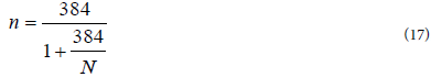
Sample size determination: The sample size for the present study was computed using formulae 1 and 2 as recommended by Bartlett et al. [62]:
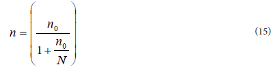
The computation of sample size for categorical data follows the same way as in continuous data, except in the computation of  , which is [62]:
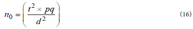
Where: p is the proportion of respondent that will give you information of interest (the proportion confirming), q viz (1-p) is the proportion not giving you information of interest (proportion defective), and p*q is the estimate of variance (which is maximum when p = 0.50 and q=0.50). The maximum population variance of 0.25 will give the maximum sample size. Consequently, the formula used to determine sample size (n) from a population (N) is:
After determining the sample size from a respective target population, a stratified random sampling techniques (using a random number table) was used to draw the respondents for the survey. First, the households were stratified into low, medium and high wealth categories and their respective percentages (of the total population) were established. Then, the sampling of respondents across the three wealth categories was affected using the following formula:
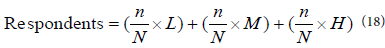
Where: n is the required sample size (calculated by equation 3), N is the households’ sampling frame, L is the number of households in a low wealth category in the sampling frame, M is the number of households in a medium wealth category in the sampling frame, and H is the number of households in a high wealth category in the sampling frame.
After the household had been selected to take part in the survey, either the husband or wife of the respective household (for a married couple) was responsible for answering the questionnaire. In the event both (husband and wife) were present at the time a visit for interview was made, then a random sampling technique (using playing cards) was used to determine who should be the respondent. Otherwise, for those households whose heads were single or at the time of the visit there was only one of the couple present, the questionnaire was administered to either single household heads or the available couple member (for the latter case).
Data collection and analysis: Data was collected using a number of techniques: household questionnaire survey, focus group discussion, key informant interview, and researcher’s direct observation. Questionnaires were both pre-tested and pilot-tested before actual data collection.
Household income determination: Household permanent income may be measured using income or consumption [63]. Whether income or consumption should be used to measure permanent income can depend on the quality and availability of survey data. Specifically, if income is traditionally underreported in surveys, then consumption may be a better measure of permanent income. Alternatively, if consumption is difficult to measure or many components of consumption are missing from the survey (or the reporting period is too short to obtain an accurate measure) income may be a preferred measure [63]. Income is notoriously difficult to measure in surveys, as respondents may be reluctant to respond to their income, and it is difficult to remember income from many different sources accurately [64,65].
In the context of this study, various working definitions were formulated as follows: Household head refers to a person responsible for day-to-day provisions for all household members. Household members mean people living and eating together for at least one month before this study was carried out. Household income is the total income from all household members with exception of maids and servants of that respective household. Table 2 shows a part of household questionnaire that was used to capture information on household income.
| Household member | Gender | Age | Marital status | Education level | Main occupation | Income/wage/salary (Tshs)* (Note: make sure you indicate if theincome is: daily/weekly/monthly/annually) |
|---|---|---|---|---|---|---|
| 1)Male 2)Female |
1)Married 2)Nevermarried 3)Widowed 4)Divorced 5)Separated |
Illiterate Primary Secondary Adult College University Others(specify) ……………………………………………………………………………………………… |
1)Employee 2)Formerly 3)employed 4)Casual labourer 5)Artisan 6)Herder/cultivator 7)Trade/shop 8)Petty business 9)Firewood/charcoal 10)Housework 11)Student Others (specify)…… |
|||
| 1.Respondent | ||||||
| 2. | ||||||
| 3 | ||||||
| n | ||||||
| *Income for every member of the household aged 18 years and above should be recorded | ||||||
Table 2:Part of household questionnaire showing how income was computed.
Data analysis: Data analysis was carried out using SPSS and Excel statistical computer programmes. Prior to detailed analysis, data were arranged in such a way as to facilitate analyses. Household income categories were collapsed from previous eight categories to three categories. Descriptive statistical analysis was conducted. The general purpose of descriptive statistical method is to summarise, organise and simplify a set of scores [30,66]. In the present study, the central tendency (average or representative score) for numeric data (interval or ratio) was determined by mean. The central tendency determination for discrete variables was a mode. The measure of variability within the numeric (interval or ratio) data was standard deviation. The categorical variables were summarised using bar charts and pie charts. Both poverty and inequality were analyses were carried out using all the reviewed approaches.
Results
Respondents’ characteristics
The socio-economic characteristics for 568 respondents who took part in the present study are summarised and presented in Table 3. The findings reveal that both household heads and those who are not household heads participated in answering survey questionnaires. It is also evident from the findings (Table 3) that the study sample comprised of both male-headed households and female-headed households, albeit the former constitutes the majority. Female-headed households can further be categorised into two groups: those who are married and those who are not. The study attained a fairly good gender balance: the number of male respondents was comparable to that of female respondents. Household income distribution for the respondents (as recorded in the field) is presented in Table 4. Figure 5 shows the distribution of the collapsed household income categories (which was used during data analysis).
Wealth status of the respondents: Prior to actual data collection, the respondents were stratified into three wealth categories (based on the criteria developed during pilot study, using focus group discussion): low wealth categories, medium wealth categories, and high wealth categories. Figure 6 indicates that the respondents constituted a fairly good representation across the three wealth category strata. During data collection, household assets were used as proxy for household wealth. Both animate (cattle, goats, sheep, pigs and chickens) and inanimate assets (land, motor cars, bicycles, hand hoes, sickles, machetes, and sprayers) were recorded for each respondent household and converted into monetary value to reflect the wealth status of a respective household. Table 5 shows the type and quantity of asserts owned by the respondents in the study area. Besides, the study sought to determine wealth ownership equity by gender.
Poverty and income inequality in the study areas
Income − poverty in the study area: The present study has striven to analyse poverty in the study area using a number of suggested thresholds in order to get a deeper insight how the different thresholds can affect the reported poverty situation in a given area. Relative poverty lines were computed using both the per-capita median income and per capita mean income at proportions of 40%, 50% and 60%. Table 6 shows the per capita household mean and median income; Table 7 presents the computed relative poverty lines; and percent of populations (respondents) below poverty lines are shown in Table 8 and Table 9.
Poverty gap ratio and poverty severity
Using the weighted geometric mean of relative poverty line (at 50% of the median) and absolute poverty line (2005PPP), both the poverty gap ratio and poverty severity were calculated. The findings indicate that both poverty gap and severity are highest in urban areas and lowest in peri-urban area (Figure 7): poverty gap and severity respectively are 0.35 and 0.29 in urban areas, 0.33 and 0.24 in rural areas; and 0.29 and 0.20 in peri-urban areas.
| Characteristic | N | % |
|---|---|---|
| Respondents | ||
| Household head | 307 | 54 |
| Not household head | 261 | 46 |
| Gender of the household head | ||
| Male-headed household | 468 | 82.4 |
| Female-headed household | 100 | 17.6 |
| Marital status of respondent | ||
| Married | 433 | 76.2 |
| Never married | 34 | 6 |
| Widowed | 67 | 11.8 |
| Divorced | 18 | 3.2 |
| Separated | 16 | 2.8 |
| Marital status of female-headed household | ||
| Married | 36 | 36 |
| Not married | 64 | 64 |
| Dwelling categories (status) | ||
| Concrete/burnt bricks/iron roof | 318 | 56 |
| Concrete/burnt bricks/grass roof | 60 | 10.6 |
| Unburnt bricks/iron roof | 18 | 3.2 |
| Unburnt bricks/grass | 9 | 1.6 |
| Mud-house/iron roof | 36 | 6.3 |
| Mud-house/grass roof | 69 | 12.1 |
| Other types | 58 | 10.2 |
| Educational level of household head | ||
| Illiterate | 99 | 17.4 |
| Primary education | 382 | 67.3 |
| Secondary education | 63 | 11.1 |
| Adult education | 3 | 0.5 |
| College education | 9 | 1.6 |
| University education | 6 | 1.1 |
| Others | 6 | 1.1 |
| Main occupation of household head | ||
| Employee | 44 | 7.7 |
| Formerly employed | 24 | 4.2 |
| Causal labourer | 7 | 1.2 |
| Artisan | 9 | 1.6 |
| Herder/cultivator | 231 | 40.7 |
| Trade/shop | 24 | 4.2 |
| Petty business | 96 | 16.9 |
| Firewood/charcoal vending | 3 | 0.5 |
| Housework | 57 | 10 |
| Others | 73 | 12.8 |
| Ownership of dwelling | ||
| Rented | 84 | 14.8 |
| Owned | 484 | 85.2 |
Table 3: Socio-economic characteristics of respondents.
| Income month-1 (Tshs) | N | % |
|---|---|---|
| < 10,000 | 80 | 14.2 |
| 10,000 – 20,000 | 86 | 15.1 |
| 21,000 – 30,000 | 55 | 9.7 |
| 31,000 – 40,000 | 50 | 8.8 |
| 41,000 – 50,000 | 55 | 9.7 |
| 51,000 – 60,000 | 44 | 7.7 |
| 61,000 – 70,000 | 19 | 3.3 |
| ≥ 71,000 | 179 | 31.5 |
| Total | 568 | 100 |
Table 4: Distribution of Household monthly income (exchange rate2007: 1US$=1,255Tshs).
| Type of Asset | Households owning | Number household-1 | ||
|---|---|---|---|---|
| N | % | Min. | Max. | |
| Animate | ||||
| Cattle | 39 | 6.7 | 1 | 250 |
| Sheep | 8 | 1.4 | 2 | 30 |
| Goats | 84 | 14.8 | 1 | 37 |
| Pigs | 53 | 9.3 | 1 | 18 |
| Chicken | 294 | 51.8 | 1 | 180 |
| Ducks | 19 | 3.3 | 2 | 15 |
| Others (e.g. pigeons) | 20 | 3.5 | 1 | 200 |
| Inanimate | ||||
| Sprayers | 6 | 1 | 1 | 2 |
| Hand hoe | 347 | 61 | 1 | 13 |
| Machete | 190 | 33.5 | 1 | 6 |
| Sickle | 28 | 5 | 1 | 5 |
| Bicycle | 211 | 37 | 1 | 26 |
| Land | 343 | 60.4 | 0.25 acre | 56 acre |
| Cars | 22 | 3.9 | 1 | 3 |
| Motor cycle | 5 | 0.9 | 1 | 2 |
Table 5: Household assets endowment in the study area.
| Stratum | Valid sample size (N) | Mean income (Tshs/month) |
Median income (Tshs/month) |
|---|---|---|---|
| Rural | 220 | 31,115.00 | 6,208.00 |
| Peri-urban | 130 | 11,440.00 | 6,250.00 |
| Urban | 97 | 29,182.00 | 10,000.00 |
| Overall | 447 | 24,974.00 | 6,666.00 |
| *Exchange rate2007: 1US$ = 1,255 Tshs | |||
Table 6: Per capita household mean and median income in the study area*.
| Stratum | Median poverty lines (Tshs/person/month) |
Mean poverty lines (Tshs/person/month) |
||||
|---|---|---|---|---|---|---|
| 40% | 50% | 60% | 40% | 50% | 60% | |
| Rural | 2,483.00 | 3,104.00 | 3,724.00 | 12,446.00 | 15,557.00 | 18,669.00 |
| Peri-urban | 2,500.00 | 3,125.00 | 3,750.00 | 4,576.00 | 5,720.00 | 6,864.00 |
| Urban | 4,000.00 | 5,000.00 | 6,000.00 | 11,672.00 | 14,591.00 | 17,509.00 |
| Overall | 2,666.00 | 3,333.00 | 4,000.00 | 9,989.00 | 12,487.00 | 14,984.00 |
| *Exchange rate2007: 1US$ = 1,255 Tshs | ||||||
Table 7: Computed relative poverty lines (using per capita household mean and median income)*.
Income inequality in the study area
In the present study, income inequality among households was determined using Gini coefficient, while inter-strata and regional inequalities were computed using both Hoover index and Theil index. The results are presented in Table 10 and Table 11.
Results
The sample of 568 households used for the present study was fairly representative in that it drew respondents from rural areas (258 respondents), peri-urban areas (177 respondents) and urban areas (133 respondents), and across subjectively established wealth categories: of all the respondents 20% were from high wealth category, 35% from low wealth category, and 45% from medium wealth category. Both household heads (54% of all respondents) and non-household heads (46% of all respondents) participated in the study. The majority of the respondents were literate (> 82%) and agrarian (> 40%). The study findings reveal that the respondents have poor assets endowment (as a proxy of wealth) which is, nevertheless, equitably owned between two genders.
Empirical evidence suggests that the majority of households in the study areas are, by the considered standards, poor. Different poverty thresholds (relative, absolute, and weighted geometric mean of relative and absolute) were used to analyse the poverty situation in the study area − in order to appreciate how subjective is the whole process of defining and quantifying the poor people. Apparently, the relative poverty thresholds using mean income were relatively higher than their counterpart thresholds using median income and consequently led to higher head counts of poor people (poverty incidence). The present study adopted 50% of the median per-capita household income as relative poverty line. Lusambo strongly favour the concept of viewing poverty in both relative and absolute terms. Consequently, in determining the incidence, depth and severity of poverty in the study area, the weighted geometric mean of relative poverty line and absolute poverty line (US$ 1-a-day at 2005 purchasing power parity) was used. Based on this poverty line, overall, 53.5% of households are poor, with rural−peri-urban−urban variations: in rural areas 55% of households are poor, in peri-urban areas 53.8% of households are poor, while in urban areas 46.4% of households are poor.
| Poverty line | Percentage (%) below poverty line | |||
|---|---|---|---|---|
| Rural area | Peri-urban area | Urban area |
Overall | |
| 1. Relative poverty line | ||||
| 1.1. 40% of the median | 24.5 | 20.0 | 37.1 | 29.3 |
| 1.2.50% of the median | 35.5 | 31.5 | 40.2 | 34.9 |
| 1.3. 60% of the median | 38.6 | 34.6 | 43.3 | 38.7 |
| 1.4. 40% of the mean | 73.2 | 38.5 | 52.6 | 59.7 |
| 1.5: 50% of the mean | 74.5 | 47.7 | 59.8 | 67.6 |
| 1.6. 60% of the mean | 76.4 | 53.1 | 62.9 | 71.1 |
| 2.Word Bank’s Absolute poverty line* | ||||
| 2.1 US$ 31/person/month (PPP 1985) (= Tshs 38,905/person/month) |
88.6 | 95.4 | 81.4 | 89.0 |
| 2.2 US$ 32.74/person/month (PPP 1993) (= Tshs 41,088.70/person/month) |
89.1 | 96.2 | 82.5 | 89.7 |
| 2.3 US$ 1.25/person/day (PPP 2005) (= Tshs 47,062.50/person/month) |
92.3 | 97.4 | 84.5 | 92.2 |
| 2.4 US$ 49/person/month (PPP 2008) (= Tshs 61,495/person/month) |
94.1 | 99.2 | 87.6 | 94.2 |
| 3. Ethical poverty line : (US$ 2,200 PPP pp pa) = (US$ 183.33 PPP pp pm) (= Tshs 287,598.90 pp pm)** |
96.8 | 100 | 99.0 | 98.2 |
| *The average exchange rate for 2007 in Tanzania was Tshs. 1,255 per 1US$ (CIAWorld Fact Book[72]). **2005PPP has been assumed |
||||
Table 8:Population below poverty lines in the study area.

Figure 5:Categories of household monthly income (exchange rate2007: 1US$=1,255Tshs).
| Stratum | Absolute poverty line | % of Median | % of Mean | ||||
|---|---|---|---|---|---|---|---|
| 40% | 50% | 60% | 40% | 50% | 60% | ||
| Rural | US$ 1-a-day (1985PPP) | 5,669.04 (48.2) | 6,627.45 (51.4) | 7,529.60 (58.6) | 17,519.75 (77.3) | 20,481.65 (79.5) | 23,269.77 (82.3) |
| US$ 1-a-day (1993PPP) | 5,762.70 (48.2) | 6,736.90 (55.0) | 7,654.00 (59.1) | 17,809.16 (77.3) | 20,820.00 (79.5) | 23,654.15 (82.3) | |
| US$ 1-a-day (2005PPP) | 6,002.20 (49.1) | 7,016.94 (55.0) | 7,972.00 (59.1) | 18,549.35 (77.7) | 21,685.30 (80.9) | 24,637.30 (82.7) | |
| Peri-urban | US$ 1-a-day (1985PPP) | 5,695.90 (47.7) | 6,658.80 (53.1) | 7,565.25 (59.2) | 8,696.87 (63.8) | 10,167.17 (66.9) | 11,551.20 (71.5) |
| US$ 1-a-day (1993PPP) | 5,789.95 (47.7) | 6,768.80 (53.8) | 7,690.20 (60.0) | 8,840.53 (63.8) | 10,335.10 (66.9) | 11,742.00 (71.5) | |
| US$ 1-a-day (2005PPP) | 6,030.60 (50.0) | 7,050.10 (53.8) | 8,009.85 (60.8) | 9,208.00 (64.6) | 10,764.68 (66.9) | 12,230.00 (72.3) | |
| Urban | US$ 1-a-day (1985PPP) | 7,914.85 (43.3) | 9,252.95 (46.4) | 10,512.50 (50.5) | 16,750.50 (61.9) | 19,582.37 (63.9) | 22,248.00 (71.1) |
| US$ 1-a-day (1993PPP) | 8,045.60 (44.3) | 9,405.80 (46.4) | 10,686.20 (50.5) | 17,027.20 (62.9) | 19,905.84 (64.9) | 22,615.55 (71.1) | |
| US$ 1-a-day (2005PPP) | 8,380.00 (45.4) | 9,796.70 (46.4) | 11,130.30 (51.5) | 17,734.90 (62.9) | 20,733.20 (69.1) | 23,555.54 (71.1) | |
| Overall | US$ 1-a-day (1985PPP) | 5,959.10 (47.0) | 6,966.55 (51.9) | 7,914.85 (55.7) | 15,020.57 (72.0) | 17,559.95 (76.3) | 19,950.34 (77.4) |
| US$ 1-a-day (1993PPP) | 6,057.50 (48.1) | 7,081.60 (51.9) | 8,045.60 (56.6) | 15,268.68 (73.4) | 17,850.00 (76.3) | 20,279.89 (79.6) | |
| US$ 1-a-day (2005PPP) | 6,309.30 (48.8) | 7,375.95 (53.5) | 8,380.00 (57.5) | 15,903.30 (73.6) | 18,591.90 (77.0) | 21,122.79 (79.6) | |
Table 9:Monthly poverty lines (and head count index in the brackets) using weighted geometric mean of relative and absolute poverty lines (ρ = 0.7).
| Location | Gini coefficient (G) |
|---|---|
| 1. Morogoro District | 0.820 |
| 2. Songea District | 0.676 |
| 3. Pooled sample | |
| 3.1 Rural areas | 0.821 |
| 3.2 Peri-urban areas | 0.574 |
| 3.3 Urban areas | 0.717 |
| 3.4 Overall | 0.773 |
Table 10: Household income inequality in the study area.

Figure 6:Wealth categories of respondents as defined during FGD.
The findings revealed further that the poverty gap ratio and severity ratio are highest in urban areas (0.35 and 0.29 respectively), medium in rural area (0.33 and 0.24 respectively) and minimum in peri-urban area (0.29 and 0.20 respectively). This is in contrast with the conclusion made by Wangwe [9], that poor people in rural areas are poorer than their counterparts in urban areas. The overarching message here is that when talking of poor people, a yardstick used to gauge them should be explicitly and objectively defined. Intuitively and using field experience, rural people are, when socially defined (i.e., access to basic services and resources), poorer than their counterparts in urban area, but the present study (based on the weighted geometric average poverty threshold) provides no empirical evidence in support of this assertion.
Methodological challenges in poverty measurements are explicitly revealed in the findings of this study. Various poverty lines were used to assess poverty situation in the study area, and each produced different results. A relative poverty line using 40%, 50% and 60% of the median income suggested that 29.3% to 38.7% of households in the study area are poor. Slightly different results were obtaining using relative poverty line of 40%, 50% and 60% the mean income: 59.7% to 71.1% of households are poor. While ethical poverty line suggested that 98.2% of households are poor, the World Bank Absolute poverty line (1993 purchasing power parity, 2005 purchasing power parity, and 2008 purchasing power parity) revealed that between 89% and 94.2% of households in the study area are poor. Further, the Weighted Geometric Mean of Relative and Absolute poverty lines (p = 0.7) suggested that using median income, 51.9% to 53.5% of households are poor; while using mean income 76.3% to 77% of households in the study area are poor. It is unequivocal, from the discussion above, that ascertaining the poverty status of a given population is not an easy task, and thus presents methodological challenges.
Household income inequality (as measured by Gini coefficient) in the study area was 0.773. Findings suggest that income inequality is highest in rural area (Gini coefficient = 0.821), medium in urban area (Gini coefficient = 0.717), and lowest in peri-urban area (Gini = 0.574). When segregated by study districts, Morogoro District manifested higher income inequality (Gini coefficient = 0.820) than Songea District (Gini coefficient = 0.676). These household income inequality values have to be interpreted cautiously as it has been pointed out by Gibson et al. [51] that when using monthly income data (cross-sectional income data), income inequality values tend to be higher by 17% to 69% than when annually collected (longitudinal) income data are used. Nevertheless, the present study seems to produce more plausibly comparable Gini coefficient values than those presented in Table 12.
Table 11 illuminates the pattern of increasing Gini coefficient values from relatively more developed countries to relatively more developing countries. In light of Table 11, the Gini coefficient value of 0.35 for Tanzania [4,67], is less plausible. Even Narayan [4] wonders whether the decline of Gini coefficient for income from 0.60 (in 1991) to 0.35 corresponds to a new path or is due to statistical and measurement error − noting that income levels particularly in rural are difficult to measure. Carter said that the value of the Gini coefficient usually varies around 0.25 in Scandinavian countries to a little over 0.6 in the most unequal economies in the developing world. The Namibia, which is regared as a middle-income country, with an annual per-capita income of US$ 2100, has a Gini coefficient of 0.7 [68]. The Namibian Government [69] reported that although Namibia has one of the higher GDP per capita, it also has one of the most unequal distribution of income and wealth in the world (Gini coefficient of 0.6 versus an average of 0.43 for all middle-income countries): over 60% of the national income is captured by the richest 10% (or less) of the population. Held and Kaya [70] posited that the Gini coefficient for the world is 0.63. Only Namibia and Lesotho have, respectively, the Gini coefficient of 0.707 and 0.632. The authors (ibid) reported further that South Africa and Brazil have the same Gini coefficient of 0.59.
The inter-regional and inter-strata income inequality was computed using both Hoover coefficient (Robin Hood index) and Theil coefficient. The findings suggest that income inequality within rural− periurban−urban continuum (Hoover coefficient = 0.158) is higher than inter-regional income inequality (Hoover coefficient = 0.116). Citing a Theil coefficient value is a bit challenging because each of the three computational formulae recommended by the literature (equation 12; 13 and 14) produced a different value. This implies that depending on the formula used, the value of the Theil coefficient for the same data set will vary − which is confusing [71]. A close scrutiny of the results indicates that the Theil coefficient computational equation 12 provided by Marsh and Schilling [40] is particularly misleading because it produces values which are beyond the upper value [i.e., log(n)] for Theil coefficients, as posited by Goodchild and Ganelle [49] and Rey and Janikas [50]. For the inter-strata inequality, the upper limit of Theil coefficient is supposed to be log (3) = 0.477, while for inter-regional inequality the upper limit of the Theil coefficient is supposed to be log (2) = 0.301.The inter-strata and inter-regional Theil coefficients of 1.519 and 1.131 respectively, fall outside the above-mentioned upper boundaries. Lusambo suggest the modification of the formula to read:
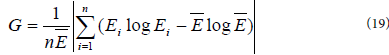
where all the variables are as previously defined. This formula has essentially changed the position of absolute value sign i.e., Using this formula provides Theil coefficients for inter-strata and inter-regional income inequality of 0.172 and 0.09 respectively, which are within their respective upper limits. The root causes of the observed poverty and income-inequality in the study area are inexplicable. The possible causes however may be one of those highlighted by Sachs [7]. Sachs [7] reported that the household income per capita can be negatively affected by a number of factors: lack of saving; absence of trade; natural resource decline (e.g. loss of soil fertility); population growth; poor technology; and adverse productivity shock (e.g. floods, drought, pests, human disease or some combination of the aforementioned factors).
| Location | Variables used | Income inequality indices | ||||
|---|---|---|---|---|---|---|
| Hoover coefficient (HC) | Theil coefficient (T) computed from various equations | |||||
| Eq.13 | Eq.14 | Eq.12 | Proposed* | |||
| Inter-strata | Rural: yi=31, 115.65 Tshs/capita =24,974.13 Tshs/capitaAi=220 Atotal= 447 |
0.158 | 0.135 | 0.035 | 1.519 | 0.172 |
| Peri-urban: yi= 11,440.79 Tshs/capita =24,974.13 Tshs/capitaAi=130 Atotal= 447 |
||||||
| Urban: yi= 29,182.39 Tshs/capita =24,974.13 Tshs/capitaAi= 97 Atotal= 447 |
||||||
| Inter-regional | Morogoro District: yi=30,299.68 Tshs/capita =24,974.13 Tshs/capitaAi=244 Atotal= 447 |
0.116 | 0.051 | 0.004 | 1.131 | 0.090 |
| Songea District: yi= 18,572.97 Tshs/capita =24,974.13 Tshs/capitaAi=203 Atotal= 447 |
||||||
| *computation based on the proposed modification (by the present study) | ||||||
Table 11: Geographical (regional) income inequality in the study area.

Figure 7:Poverty gap ratio and severity in the study area.
| S. No | Region | Average Gini coefficient |
|---|---|---|
| 1. | Latin America and Caribbean | 0.4978 |
| 2. | Sub-Saharan Africa | 0.4605 |
| 3. | Middle East and North Africa | 0.4049 |
| 4. | East Asia and the pacific | 0.3875 |
| 5. | South Asia | 0.3508 |
| 6. | Industrial countries and high income developing countries | 0.3431 |
| 7. | Eastern Europe | 0.2657 |
| Source: Modified from Bhorat[71] | ||
Table 12: Gini coefficient estimate over four decades (1960s, 1970s, 1980s and 1990s).
Sachs [7] posited that at the most basic level, the key to ending extreme poverty is to enable the poorest of the poor to get their feet on the ladder of development, noting that the extreme poor lack six major kinds of capital: human capital (health, nutrition and skills); business capital (machinery, facilities, motorised transport used in agriculture, industry and services); infrastructure (roads, power, water and sanitation, airports and seaports, and telecommunication systems that are critical inputs into business productivity); natural capital (arable land, healthy soil, biodiversity, and well functioning ecosystems that provide the environmental services needed by human society); public institutional capital (commercial law, judicial systems, government systems and policing that underpins the peaceful and prosperous division of labour); and knowledge capital (the scientific and technological know-how that raises productivity in business output and the promotion of physical and natural capital) [72-74].
Conclusions
This paper has analysed the respondents’ characteristics in detail, putting a special emphasis on their poverty situation. Albeit crosssectionally studied, empirical evidence indicates that the majority of households in the study area are under the poverty line by any reasonable standard. High income (monetary) inequality among the households has been revealed. Inequality among geographical locations (inter-strata and inter-regional) is significantly less than that among households − with the inter-regional inequality being the least.
Different poverty lines have provided different results regarding the number of households which are poor. Relative poverty line of 40% of the median income gave the lowest value of poverty in the study area, while the ethical poverty line provided the highest rate of poverty. Accordingly, it was found that using selected poverty lines: overall, 29.3% - 98.2% of households are poor. In rural areas, 24.5% - 96.8% of households are poor. In peri-urban areas, it was found that 20% to 100% (depending on the poverty line used) were poor, while in urban areas the poverty rate was found to be between 37.1% to 99%. Using weighted geometric mean of relative and absolute poverty lines (ρ = 0.7) at relative poverty line of 50% of median income and absolute poverty line of US$ 1-a-day (2005PPP): Overall, 53.5% of households are poor, and poverty rates in rural, peri-urban and urban areas are 55%, 53% and 46% respectively.
When reporting on poverty aspects − incidence, depth and severity − an explicit description of a yardstick used in gauging the poor is imperative. This is so because, as evidenced by the present study, the process of defining and subsequently quantifying the poor is, in a way, subjective and primarily dependent on the yardstick used. Literature has favoured the use of Theil coefficient as a metric for analysing regional resource inequality (resource concentration). The empirical evidence has revealed a high level of subjectivity among the recommended computational formulae for this coefficient: apparently each formula, when applied on the same data set, results in a different value of the coefficient.
Household income inequality in the study area is high (Gini Coefficient = 0.773), with variations in the strata as follows: rural areas (Gini Coefficient = 0.821); peri-urban areas (Gini Coefficient = 0.574); and urban areas (Gini Coefficient = 0.717). Inter-strata inequality index in the study area (depending on the method used) ranged between 0.158 – 0.172, while inter-regional inequality index ranged between 0.004 and 0.116.
The empirical poverty incidence in the study area (for 2007) is at variance with the recently reported one (by Tanzanian government through its Ministry of Finance and Planning) using the Tanzanian national poverty line. Though is improper to compare the two rates of poverty incidence (since they are based on different yardsticks), the rate reported by the government (for 2007) seems to be understated. This may have perilous consequences on the under-way poverty alleviation efforts as well as the future ones. The gravity of poverty problems needs to be properly and accurately determined so that appropriately commensurate efforts can be launched against it.
Recommendations
The Millennium Development Goal (MGD) number one strives to eradicate extreme poverty and hunger. It is therefore imperative that the gravity of poverty problems needs to be properly and accurately determined so that appropriately commensurate efforts can be launched against it. The yardstick used to determine poverty rate need to be objective and consistent so as to enable reasonable comparability of poverty situation between different communities and/or nations. This study recommends the following:
Firstly, in the determination of poverty rates (head counts) the appropriate yardstick to be used is weighted geometric mean of relative and absolute poverty lines (ρ = 0.7) at relative poverty line of 50% of median income and absolute poverty line of US$ 1-a-day (2005PPP). This yardstick is more reasonable because it considers both relative and absolute poverty lines in determining how many people/households are poor. As depicted by the study findings, this yardstick revealed the expected patterns of decreasing poverty rates from rural areas to urban areas.
Secondly, in the determination of household income inequality, Gini Coefficient should be used. The suitability of this yardstick has been highlighted also by various authors: Habibov and Fan [46] and World Bank [47] reported that in measuring inequality, Gini Coefficient is one of the most commonly used measure, and that using Gini Coefficient has advantage insofar as it satisfies three important principles, which are. Anonymity: it does not take into account who the wealthy and poor are. Scale Independence: it does not take into account the size of the economy, wealth of the country, and the size of population in the country. Transfer Principle: if income is transferred from the wealthy to the poor, the Gini Coefficient demonstrates more income distribution.
Thirdly, the Hoover coefficient (Robin Hood Index) is a more appropriate metric for regional and inter-strata inequality because it is more explicit and devoid of this anomaly exhibited by Theil coefficient as a metric for analysing regional resource inequality (resource concentration). The empirical evidence has revealed a high level of subjectivity among the recommended computational formulae for this coefficient: apparently each formula, when applied on the same data set, results in a different value of the coefficient.
Acknowledgement
I owe so much-and therefore am exceedingly grateful - to my supervisor Prof. Colin Price for his outstanding guidance, advice, assistance, encouragement and constructive criticism throughout the study. I wish to register my gratitude to Prof. Y.M. Ngaga of Sokoine University of Agriculture (SUA), Tanzania, for his assistance in shaping my study theme and subsequently editing my questionnaires prior to field work data collection. I am indebted to my employer, the Sokoine University of Agriculture for granting me the study leave and Association of Commonwealth University Sponsorship for financing my studies and the British Council for effectively administering the scholarship. Prof. Ric Coe’s guidance on statistical issues to my study during his two consecutive visits to Bangor University was too invaluable to go unappreciated. I will invariably cherish his contribution to my success. I also express my gratitude to Dr. John. B. Hall for his encouragement and constructive comments during my final thesis write-up.
My heart-felt gratitude also go to the WWF for their partial financial support during fieldwork, without which data collection would be absolutely difficult undertaking due to my then financial constraints for fieldwork. Successful data collection also hinged on diligent and devoted fieldwork assistants who painstakingly rendered their assistance in collecting quality data. I will thus not do them justice if I don’t acknowledge them. I would like to thank the Morogoro and Songea-District Administrative Secretaries for permitting me to carry out my study in areas under their jurisdiction. Thanks also go district forest officials, ward executive officers (W.E.O), Village executive officers (V.E.O) and hamlet/street leaders for their invaluable support during the entire period of data collection. I am highly indebted to all respondents in the study area including but not limited to households, fuel vendors, charcoal stove producers and vendors. Their cordial cooperation rendered to me during data collection is highly appreciated.
Last but not least, I’m grateful to Dr. Suzana Augustino and her husband Revocatus Nyefwe who warmly welcome me the first time I arrived at Bangor, thereby healing my homesickness. I will always remember their kindness. Special regards go to Dr. James Walmsley and my colleagues PhD students: Sally, Pete, Paul, Elizabeth, Jacob, Refaat, and Betty Waized, to name but a few, for their miscellaneous contributions to the success of my studies.
References
- May J, Sulla V, Zikhali P (2016) South African poverty and inequality assessment discussion note, World Bank, South Africa, pp: 33.
- UNDP (2006) Poverty in Focus. What is poverty? concepts and measures. International Poverty Centre.
- Organisation for Economic Cooperation and Development (OECD) (2013) Roundtable discussion on competitions and poverty reduction.
- Narayan D (1997) Voices of the poor: Poverty and social capital in Tanzania. World Bank Publications, pp: 80.
- Handley G, Higgins K, Sharma B, Bird K, Cammack D (2009) Poverty and poverty reduction in Sub-Saharan Africa: An overview of the issues. Results of ODI Research presented in preliminary form for discussion and critical comments. Working Paper 299. OverseasdevelopmentInstitute (ODI), London.
- Madulu NF (2003) Linking poverty levels to water resources use and conflicts in rural Tanzania. Physics and Chemistry of the Earth Parts A/B/C 28: 911-917.
- Sachs JD (2005) Who and where are the poor?
- Duclos J, Araar A (2006) Poverty and equity: measurements, policy and estimation with DAD. In: Jacques S (ed.) Economic studies in inequality, social exclusion and well-being, Springer, New York, pp: 416.
- Wangwe SM (1997) Economic reforms and poverty alleviation in Tanzania. Economic and Social Research Foundation, Dar es Salaam, Tanzania, pp: 79.
- Carrasco E, García-Grimeno R, Seselovsky R, Valero A, Pérez F, et al. (2006) Predictive model of listeria monocytogenes’ growth rate under different temperatures and acids. Food SciTechnolInt 12: 47-56.
- Frye I (2005) Constructing and adopting an official poverty line for South Africa: some issues for consideration. A discussion document. National Labour and Economic Development Institute, South Africa.
- Blackorby C, Donaldson D (1980) Ethical indices for the measurement of poverty. Econometrica 48: 1053-1060.
- Saunders P, Smeeding T (2002) Beware the mean! Social Policy Research Centre Newsletter No.81, Sydney, Australia, pp: 12.
- Arnold JEM (2001) Forestry, poverty and aid. Occassional Paper No 33. Center for International Forestry Research (CIFOR). Bogor, Indonesia, pp: 17.
- Ortiz I, Daniels LM, Engilberts D (2012) Child poverty and inequality: new perspectives. United Nations’ Children Fund (UNICEF), Division of Policy and Practice. New York, pp: 1-299.
- Smeeding T (2006) Poor people in rich nations. The United states in comparative perspective.J Econ Perspect 20: 69-90.
- Jesuit D, Smeeding T (2002) Poverty levels in developed world. Luxembourg Income Study working paper No. 321.
- Mualuko NJ (2007) The issues of poverty in the provision of quality education in Kenyan secondary schools. Educational Research and Review 2: 157-164.
- Helwege A, Birch MBL (2007) Declining poverty in Latin America? A critical analysis of new estimates by international institutions. Global development and Environmental Institute Working Paper No.07-02, Tufts University, USA.
- Martin M (2004) Globalization, macro-economic stabilization, and the construction of social reality: An essay in interpretive political economy. LIT Verlag Berlin-Hamburg-Münster, pp: 471.
- Morris E (2008) Poverty and Inequality: The public challenge. International Institute for the study of Cuba, UK.
- Roe K (2006) Sub-Saharan Africa and extreme poverty. Paper presented at NACSW (North America Association of Christian in Social Work) Convention, Philadelphia.
- Pogge T (2008) Consistent measure of real poverty: A reply to Ravallion. International Poverty Centre, One Pager, pp: 54.
- Ravallion M, Chen S, Sangraula P (2009) Dollar a day revisited. World Bank Econ Rev 23: 163-184.
- Edward P (2006) The ethical poverty line: A moral quantification of absolute poverty line. Third World Quarterly 27: 377-393.
- Ghai D (2003) Decent work: concept and indicators. International Labour Review 142: 113.
- U S Census Bureau (2007). Income, poverty and health insurance coverage.
- Long AS (1999) Country paper on poverty measurement. The case of Singapore. Singapore Department of Statistics.
- http://www.slideserve.com/alpha/poverty-as-a-social-phenomenon-policies-of-social-security
- Gravetter FJ, Wallnau LB (2006) Statistics for the behavioural sciences(6thedn.). Academic Internet Publishers, USA, pp: 104.
- Madden D (2000) Relative or absolute poverty lines: a new approach. Review of Income and Wealth, 46: 181-199.
- Foster JE (1998) Absolute versus relative poverty. The American Economic Review 88: 335-341.
- Simler KR, Arndt C (2007) Poverty comparisons with absolute poverty lines estimated from survey data. Review of Income and Wealth 53: 275-294.
- Delamonica EE, Minujin A (2007) Incidence, depth and severity of children in poverty. Social Indicator Research 82: 361-374.
- Son HH, Kakwani N (2006) Measuring the impacts of price changes on poverty. International Poverty Centre, United Nations Development Programme.
- Werling J (2008) Inequality and poverty. Department of Economics, University of Maryland, Maryland, USA.
- Quah JKH (2006) Weak axiomatic demand theory. Economic Theory 29: 677-699.
- Jacobson A, Milman AD, Kammen DM (2005) Letting the (energy) Gini out of the bottle: Lorenz Curves of cumulative electricity consumption and Gini coefficients as metrics of energy distribution and equity. Energ Policy 33: 1825-1832.
- Bideleux R, Lunden T (2007) Europe from exclusive borders to inclusive frontiers. In: Delanty G, Pantea D, Teperics K (eds.). Journal of the Institute for Euregional Studies 4: 1-195.
- Marsh MT, Schilling DA (1994) Equity measurement in facility location analysis: A review and framework. Eur J Oper Res 74: 1-17.
- Portnov BA, Felsenstein D (2005) Measures of regional disparity for small countries. Advances in Spatial Science. Springer Berlin Heidelberg, pp: 47-62.
- Dixon PM, Weiner J, Mitchell-Olds T, Woodley R (1987) Bootstrapping the Gini Coefficient of Inequality. Ecology 68: 1548-1551.
- Damgaard C, Weiner J (2000) Describing Inequality in Plant Size or Fecundity. Ecology 81: 1139-1142.
- Burkey ML (2006) Measuring income inequality: The lorenz curve and the gini coefficient. North Carolina Agricultural and Technical State University, USA.
- Dixon PM, Weiner J, Mitchell-Olds T, Woodley R (1988) Erratum to 'Bootstrapping the Gini Coefficient of Inequality. Ecology 69: 1307.
- Habibov NN, Fan L (2006) Social assistance and challenges of poverty inequality in Azerbavijan, a low-income country in transition. The Journal of Sociology and Social Welfare 33: 203-226.
- World Bank (2013) Inequality in focus. Poverty reduction and equity department 2: 1-8.
- De Maio FG (2007) Income inequality measure. J Epidemiol Community Health 61: 849-852.
- Goodchild MF, Anselin L, Appelbaum RP, Harthorn BH (2000) Towards spatially integrated social science. International Regional Science Review 23: 139-159.
- Rey SJ, Janikas MV (2005) Regional convergence, inequality and space. Journal of Economic Geography 5: 155-176.
- Gibson J, Huang J, Rozelle S (2001) Why is income inequality so low in China compared to other countries? The effects of household survey methods. Economic Letters 71: 329-333.
- Bakar KS (2007) Trade and income inequality in SAARC: A spatial analysis. Institute of Statistical Research and Training, University of Dhaka, Bangladesh.
- Wilson I (2002) Some practical sampling procedures for development research. Statistical services centre, University of Reading, UK. A paper presented at a conference on Combining Qualitative and Quantitative Methods in Development Research, held at Centre for Development Studies, Swansea University.
- Carissa W, Marlene R, Duraiappah AK (2005) Connecting poverty and ecosystem services. A series of seven country scoping studies. Focus on Tanzania. United Nations Environment Programme (UNEP) and International Institute for Sustainable Development (IISD), pp: 1-33.
- Iraossi G (2006) The power of survey design: A user's guide for managing surveys, interpreting results, and influencing respondents. The World Bank, Washington, D.C.
- Schwab DP (1998) Research methods for organisational studies(9thedn.). Mahwah, N.J: Laurence, Erlbaum Associates.
- Barribeau P, Butler B, Corney J, Doney M, Gault J, et al. (2005) Survey Research. Writing@CSU. Colorado State University.
- Dunn KA, Huss HF, Robinson JM (2004) Mail survey reliability through follow-up mailings: the case of auditor changes. Managerial Auditing Journal 19: 1048-1054.
- Assche SB, Reniers G, Weinreb AA (2003) An assessment of the KDICP and MDICP data quality: Interviewer effects, question reliability and sample attrition. Demographic Research 2: 31-76.
- Bushery JM, Brick JM, Severynse J, McGuiness RA (1996) How interview mode affects data reliability. US Bureau of Census, Washington, DC, pp: 600-603.
- Kennet J, Painter D, Hunter SR, Granger RA, Bowman KR (2005) Assessing the reliability of key measures in the national survey on drug use and health using a test-retest methodology. Data Sharing for Demographic Research.
- BartlettJE,KotrlikJW,HigginsCC(2001)Organizational research: determining appropriate sample size in survey research. Inftechnol learn perform J 19:43-50.
- Wolff EN (2004). What has happened to the quality of life in the advanced industrialised nations? Edward Elgar Publishing, UK, pp: 392.
- Meyer MH, Daniele EA (2016) Gerontology: changes, challenges and solutions. Social Science pp: 671.
- Slemrod J, Bakija JM (2004) Taxing Ourselves: A citizen’s Guide to debate over taxes (4th Edition). MIT Press, Business and Economics, Pp: 382.
- Gravetter FJ, Wallnau LB (2007) Fundamental statistics for the behavioural sciences. 7th edition. Wadsworth Cengage Learning, USA.
- URT (2003) Poverty reduction strategy. The 2nd Progress Report 2001/02.
- Smit P (2004) A statement by Hon Paul Smit, Deputy Minister for Agriculture, Water and Rural Development of the Republic of Namibia at the 27th IFAD Governing Council Session, Rome.
- Namibia Government (2007) Country paper for the International Conference on Development Cooperation with middle-income countries, Office of the President National Planning Commission, Madrid, Spain.
- Held D, Kaya A (2007). Global inequality: patterns and explanations. Polity Press, UK and USA, pp: 273
- BhoratH(2005)Poverty, inequality and labour market in Africa: descriptive overview. Development Policy Research Unit Working Paper No. 05/92,pp: 26.
- Central Intelligence Agency CIA (2008)Tanzania economy 2008. World Fact Book.
- RadhakrishnaRB(2007)Tips for developing and testing questionnaires/instruments. Journal of Extension 45.
- RidgeJB(2010)Evaluation techniques for difficult to measure programmes: for education, non-profit, grant funded, business and human service Programmes, pp: 269.
Relevant Topics
- Aquatic Ecosystems
- Biodiversity
- Conservation Biology
- Coral Reef Ecology
- Distribution Aggregation
- Ecology and Migration of Animal
- Ecosystem Service
- Ecosystem-Level Measuring
- Endangered Species
- Environmental Tourism
- Forest Biome
- Lake Circulation
- Leaf Morphology
- Marine Conservation
- Marine Ecosystems
- Phytoplankton Abundance
- Population Dyanamics
- Semiarid Ecosystem Soil Properties
- Spatial Distribution
- Species Composition
- Species Rarity
- Sustainability Dynamics
- Sustainable Forest Management
- Tropical Aquaculture
- Tropical Ecosystems
Recommended Journals
Article Tools
Article Usage
- Total views: 20244
- [From(publication date):
June-2016 - Apr 02, 2025] - Breakdown by view type
- HTML page views : 18900
- PDF downloads : 1344