Genotype by Environment Interaction of Sugarcane (Saccharum officinarum L.) for Sugar Yield Based on GGE-Biplot and AMMI Analyses in Ethiopia
Received: 01-Dec-2023 / Manuscript No. acst-23-122555 / Editor assigned: 04-Dec-2023 / PreQC No. acst-23-122555 / Reviewed: 18-Dec-2023 / QC No. acst-23-122555 / Revised: 22-Dec-2023 / Manuscript No. acst-23-122555 / Published Date: 29-Dec-2023
Abstract
The first goal of plant breeders in crop improvement is to develop genotypes with high yield and stable across environments. AMMI and GGE-bilpot are the most effective statistical tools for the analyses of stability, adaptability and helps for proper selection of sugarcane genotypes. The present investigation was carried out on eight introduced sugarcane genotypes excluding two standard checks for three cropping cycles at Finchaa and Metehara forming together six environments. The trial was laid out in completely randomized block design. This work was conducted with objective of evaluating G x E interactions on sugar yield performances of sugarcane genotypes using AMMI and GGE statistical tools. The results of combined ANOVA and AMMI analysis of variance for sugar yield showed that highly significant (p ≤ 0.001) difference among genotypes and environments and their interactions. The sugar yield of the genotype was influenced by environments which explained 73.77% of the total variation indicating the importance of environmental main effects over genotypic main effects. The first-IPCA1 (59.08%) showed highly significant level whereas the second-IPCA2 (18.66%) were not significant and totally explained 77.74% of the variations. The analysis of the AMMI resulted that genotypes G10 (1.928), G2 (1.744), G9 (1.683) and G4 (1.633) had high mean sugar yield in ton/ ha/month. The GGE-biplot analysis grouped the environments into two mega-environments and sub-divided the graph into five sectors. The first mega-environment was made up by three environments: E1, E2 and E4 while the second mega-environment was made up by E3, E5 and E6. G2 and G10 was located very nearest to the concentric circle; thus, considered to be ideal the genotype and therefore identified as the best genotype than the others. Consequently, these two genotypes could be selected for verification and recommended for commercialization
Keywords
AMMI; GGE-Biplot; Mega-environment; Ideal genotype
Introduction
Sugarcane is a field crop plant mainly having high G x E interaction and high heterozygosity (Tena et al., 2019). The production of sugarcane is affected by the environment, genotype and the interaction of both effect (GEI); of which the GEI effect causes significant variations in cultivar performance between different locations (Mohammadi et al. 2007). Sugarcane is a vegetatively propagated crop through the planting of segments of the cane stalk called sett which contains viable buds (Smit et al., 2004). A number of genotypes are evaluated over several cropping cycles and locations for selecting superior adaptable cultivars with high stability across environments for sustainable production of sugarcane in sugar industry. Multiple environment tests of the cultivar are an essential tool because of the presence of genotype and environment interactions [1].
In crop improvement, the ambition of plant breeder is to develop genotypes with high yield and stable in different environments and then, identify locations and genotypes that best represents the target factors (Luquez et al. 2002; Ahmadi et al. 2015). Consequently, it is essential that breeders are aware of the nature of G x E interactions as well as the extent of test site similarity within a multi-environmental test as this can bring change in rankings of varieties across environments [2].
There are many statistical tools to deal with multivariate analysis having a set of data in multi environment trials. Among these, agronomist and plant breeders uses AMMI (additive main effects and multiplicative interaction) (Yan et al., 2000) and GGE (genotype main effects in addition to genotype by environment interaction biplots) (Yan et al., 2007; Yan and Kang 2003) (Jamshidmoghaddam and Pourdad, 2011) which is the most effective for the analyses of stability, adaptability and ranking of genotypes and helps for proper selection of genotypes with suitable mega environments. Both of these statistical tools integrate principal component analysis (PCA) and biplot for the explanation of genotype by environment interaction (G×E) [3].
The AMMI model combines the conventional ANOVA for the genotype main effects and environment main effects and the principal component analysis (PCA) with multiplicative factors in a single analysis. Then, it investigates the residual multiplicative interaction between genotypes and environments to determine the sum of squares of the G × E interaction (Purchase et al. 2000) and thereby helps the breeder to identify genotypes with better performance for giving judgment (Gauch et al., 1997; Tena et al., 2019). The GGE represents the main effect of genotype (G) plus the genotype by environment interaction (GE). Based on principal components analysis GGE biplot model displays the two sources of variation G and GE. It is multivariate analytical method which contains a set of biplot interpretation models concerning various data about genotype and test-environment. This model provides an adequate graphical tool for cultivar evaluation (yield and stability), mega-environment analysis(such as ‘which-won-where’ pattern), with the scores of the genotypes and the environments of the PC1 scores against their respective scores for the PC2 scores (Burgueno et al., 2009; Crossa et al., 2002; Ding et al., 2009; Yan and Kang 2003) when many genotypes are tested across locations for more than one year and/or cropping cycles(Yan et al. 2007; Vaezi et al., 2017) [4,5].
The users always need the varieties that with high yield performance and other essential agronomic traits in commercial crop production. In most cases, in Ethiopia, the sugarcane varieties under use in a commercial farm as well as under the research are introduced from foreign countries. Besides, the locations in which these cultivars tested are also vary in soil fertility, temperature range and irrigation types. Thus, statistical evaluation of this genotype is fundamental to identify the response of genotypes in relation to the environments of the experimental conditions. Therefore, it is important to understand the causes of GEI for the determination of high-yielding genotypes and identifies sites that best represent the target environment. The objective of this study was to evaluate G x E interactions of sugarcane genotypes for sugar yield across six environments using AMMI and GGE biplot models and identify genotypes with high yield and stable performance [6].
Materials and Methods
Experimental site
The experiment was conducted at two most popular sugar estates of Ethiopia; Finchaa and Metehara. Finchaa was located at latitudes 90 30’N to10000’N and longitudes 370 15’ to 370 30’E and an elevation between 14550-1600 m.a.s.l. An average annual precipitation of the area reaches about 1309 mm and the average maximum and minimum temperature was 31.50C and 14.60C respectively. Metehara sugar estate was located at latitude 80 53’ N and longitudes 390 52’ E and at an elevation of 950 meters at sea level. It receives an average of 554mm annual rainfall with minimum and maximum temperature of17.40c and 32.60c respectively [7].
Plant Materials
Eight introduced sugarcane genotypes and two commercial standard checks were evaluated at Finchaa and Metehara sugar estate. These genotypes were labeled as G1, G10, G2, G3, G4, G5, G6, G7, G8 (first standard check) and G9 (second standard check) [8].
Experimental design
The trial was laid out in randomized completely block design with three replications. The completion of the experimental period involving three crop cycles (i.e. plant cane, first and second ratoon crops) takes about four years as a single season lasts over fourteen months. The data for sugar yield and related components were collected during the crop cycles at a regular schedule at both sites. The two locations consisting of a total of six environments (sites-x-crops combinations) designated by E1-to-E6 (Table 1). Except the treatments and environments, all agronomic management practices were applied uniformly throughout the growing season as per the practice of the respective sugarcane estates [9].
| Codes for crop cycles, site, environment and year of implementation | |||
|---|---|---|---|
| crop cycles Vs Site | Combination of Crop cycles Vs Site Code | Environment | Year of the crop cycles implemented |
| Code | |||
| Finchaa (site one) | S1(code of site one) | ||
| Metehara (site two) | S2 (code of site two) | ||
| Plant cane at Finchaa | S1Pc | E1 | 2014/15 |
| First ratoon crop at Finchaa | S1R1 | E2 | 2016/17 |
| Second ratoon crop at Finchaa | S1R2 | E3 | 2017/18 |
| Plant cane at Metehara | S2Pc | E4 | 2014/15 |
| First ratoon crop at Metehara | S2R1 | E5 | 2016/17 |
| Second ratoon crop at Metehara | S2R2 | E6 | 2017/18 |
Table 1: The combinations of crop cycle with site code, environment code and year of the experiment implemented.
Statistical analysis
The collected data from the six environments (the combination of two locations and three crop cycles) were subjected to statistical analysis by General Linear Models (GLM) Procedure using SAS (SAS, 2002) and combined ANOVA was done to determine the significance level of genotype, environment and G×E interaction effects at each location and across location (Team, 2020). The genotypes and the environments were considered as a fixed and random variables respectively [10].
AMMI model is effective in partitioning the total sum of squares into genotype main effect, environment main effect and the G × E interactions (GEI), however it does not provide full information for the GEI structure. This component is dealt with more advanced techniques such as principal component analysis (PCA) of the interaction residuals after the main effects are removed (Zobel et al., 1988; Gauch, 1992) [11].
The AMMI model analysis used to estimate yield of genotype, environment and G X E interaction:
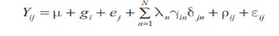
Where Yij is the value of the ith genotype in the jth environment; μ is the grand mean; gi is the deviation of the ith genotype from the grand mean(genotype main effect); ej is the deviation of the jth environment from the grand mean(environment main effect); Ν is the number of IPCA retained in the model; λn is the eigen value of the nth interaction principal component analysis (IPCA) retained in the AMMI model; ϒin is the eigen vector for the ith genotype from nth IPCA; δjn is the eigen vector for the jth environment from the nth IPCA; ρij is the GE interaction residual; Ɛij is the random error term [12].
The GGE-biplot is composed of the biplot (Gabriel, 1971) and the GGE (Yan et al. 2000) concepts. It uses a biplot to show the factors (genotype and genotype x environment interaction) that are important in genotype evaluation and that are also sources of variation in GEI analysis (Yan, 2001; Yan et al., 2000). It was constructed from the first two principal components (PC1 and PC2) derived by subjecting the environment centered yield data (which contains G and GE) to singular valued composition [13].
The sums of squares of a PCA axis are termed its “eigenvalue”, and its direction relative to the original axis system is termed its “eigenvector” (Sanesh, 2012). The AMMI and GGE biplot analyses were done using Genstat software (International, 2009). The GGE-biplots and AMMI are graphical images to exemplify G × E interaction and genotype ranking based on mean and stability (Zobel et al., 1988). The graph generated is based on multi environment evaluation yield trial (whichwon- where pattern). Genotype evaluation (mean versus stability), and the environment are tested by their ranking (discriminative versus representative) [14].
Result and Discussions
AMMI analysis of variance
The results of combined ANOVA and AMMI analysis of variance for sugar yield showed that highly significant (p ≤ 0.001) difference among genotypes (G), environments (E) and genotype by environment interaction (GEI). Based on the AMMI result, the sugar yield of the genotype were influenced by environments which explained 73.77% of the total phenotypic (G + E + GEI) variation while the genotype (G) and genotype by environment interaction (GEI) accounted 8.65% and 17.58% respectively indicating the contribution of environmental main effects over genotypic main effects for the variation of sugar yield due to diverse environmental conditions of the testing locations. Similar to this result, the higher donation of environment than the genotype and their interaction was reported in sugar yield by Tena et al. (2019) and by Legesse et al. (2019) in grain yield of maize [15]. The magnitude of sum squares of GEI is greater than that of genotype effects, indicating that there are more differences in genotypic response across environments. This result was not confirm with Erol et al. (2018) that reported the highest genotypic effect than GEI in the study undertaken for the selection of the best barley genotypes to multi and special environments by AMMI.
The GE interactions effect in the AMMI model has been partitioned into two Interaction Principal Component Axes (IPCA1 and IPCA2) [16]. The first-IPCA1 showed highly significant level whereas the second-IPCA2 were not significant recording 59.08%, and 18.66%, respectively with a decrease in the subsequent axes and totally explained 77.74% of the variations observed. The rest 22.26% of the interaction effect was residual, therefore, not interpreted (Purchase et al., 2000). The significance level of the first-IPCA1 indicates that the sugarcane clones and the six environments were considerably different from one another. This end result was in agreement with Vaezi et al. (2017) and Regis et al. (2018). According to Legesse et al. (2019), such research result shows the performances of the genotypes used were varied differently in sugar yield (Table 2) [17].
Source |
DF | S.S. | M.S. | v.r. | F pr | % TSS Explained | % trt | % GIE explained |
|---|---|---|---|---|---|---|---|---|
| Treatments | 59 | 67.71 | 1.14*** | 7.96 | <0.001 | 79.3 | ||
| Genotypes(G) | 9 | 5.86 | 0.65*** | 4.51 | <0.001 | 8.65 | ||
| Environments(E) | 5 | 49.95 | 9.99*** | 57.04 | <0.001 | 73.77 | ||
| Block (Env) | 12 | 2.1 | 0.17 | 1.21 | 0.2825 | 2.46 | ||
| Interactions(GEI) | 45 | 11.9 | 0.26** | 1.83 | 0.0057 | 17.58 | ||
| IPCA 1 | 13 | 7.03 | 0.54*** | 3.76 | <0.001 | 59.08 | ||
| IPCA 2 | 11 | 2.22 | 0.20ns | 1.4 | 0.182 | 18.66 | ||
| Residuals | 21 | 2.65 | 0.12 | 0.87 | 0.626 | 22.26 | ||
| Error | 108 | 15.57 | 0.14 | 18.24 | ||||
| Total | 179 | 85.38 | 0.47 | |||||
| ***= highly Significant at 0.001;**= Significant at 0.01; ns= non-significant; DF = Degrees of freedom; SS = Sum of squares; MS = Mean square; TSS= Total Sum of squares; trt= treatment | ||||||||
Table 2: Combined AMMI analysis of Variance on sugar yield of the 10 sugarcane lines across six environments (the combination of two sites for three cropping cycles).
Mean performance of genotypes
The sugar yield mean values of an introduced sugarcane genotypes ranged from 1.282 to 1.928ton/ha/month. Appropriated harvesting time of the genotypes across locations had its own yield advantage in sugarcane production; hence the unit measure ton per hectare per month is used in this result. Analysis of the AMMI indicated that genotypes G10 (1.928), G2 (1.744), G9 (1.683) and G4 (1.633) had high mean sugar yield in ton/ha/month while G6 (1.282), G7 (1.336) and G5 (1.488) were the least sugar yield. The standard check genotype G9 (the second standard check) either at par or surpassed most of the tested new genotypes except G10 and G2. The genotype labeled by G10 observed to be the highest sugar yield mean value in ton/ha/month in four environments: E1, E2, E3 and E4 and also considered as the first cultivar among the first four AMMI selections for these sites [18].
Genotypes and/or environments with large IPCA1 scores (either positive or negative) have high interactions, whereas genotypes or environments with low IPCA1 scores show low contribution to the G×E interaction (Crossa et al., 1990; Oliveira et al., 2014). Accordingly, based on the first IPCA1 which scored 59.08% of sum squares of the interactions, G6 (0.081), G1 (-0.129) and G2 (-0.149) showed the lowest GEI interaction of the ten genotypes evaluated in six environments as listed in. Thus, these genotypes were considered as stable genotypes but except G2 the others two gave the lower sugar yield mean value in ton/ ha/month. On the other hand, G3 (0.698) followed by G4 (-0.641), had the largest GE interaction and are responsive to environmental change and therefore not considerably stable [19].
Moreover, an average environmental sugar yield mean values over locations varied from 0.935(E4-plant cane at Metehara) to 2.369 (E1- plant cane at Finchaa). AMMI biplot analysis showed that the least first IPCA value of 0.040 was recorded for E3 (second ratoon at Finchaa) while the highest IPCA value (0.830) was observed for E1 (plant cane at Finchaa) indicating that low interaction of the climatic conditions at E3 and high interaction at E1. Therefore, E3 was contributed more for the stability of the genotypes. The genotypes with greater IPCA score is the more openly adapted to a specific location [20]. The genotype with IPCA score approximate to the nearest to zero is the more stable and or adapted to in overall environment (Alberts, 2004; Legesse et al. 2019). However, the sugar yield of genotypes could be changed depending on the nature of its genetic make-up; while the yield of environments could display variations based on the edapho climatic conditions (Tables 3 and 4).
| Genotype Label | Genotype Mean | IPCAg[1] | IPCAg[2] | AMMI-estimates per environment † | |||||
|---|---|---|---|---|---|---|---|---|---|
| E1 | E2 | E3 | E4 | E5 | E6 | ||||
| G1 | 1.527 | -0.129 | -0.534 | 2.198 | 2.249 | 1.513 | 0.546 | 1.205 | 1.453 |
| G10 | 1.928 | 0.432 | -0.048 | 3.082 | 2.775 | 1.547 | 1.278 | 1.445 | 1.443 |
| G2 | 1.744 | -0.149 | 0.238 | 2.4 | 2.241 | 1.377 | 1.251 | 1.699 | 1.498 |
| G3 | 1.51 | 0.698 | 0.328 | 2.897 | 2.378 | 0.886 | 1.109 | 0.998 | 0.792 |
| G4 | 1.633 | -0.641 | 0.073 | 1.899 | 1.965 | 1.456 | 1.016 | 1.795 | 1.665 |
| G5 | 1.488 | 0.164 | 0.218 | 2.428 | 2.144 | 1.046 | 0.995 | 1.241 | 1.071 |
| G6 | 1.282 | 0.081 | 0.12 | 1.15 | 1.927 | 0.907 | 0.725 | 1.052 | 0.933 |
| G7 | 1.336 | -0.277 | 0.063 | 1.905 | 1.837 | 1.076 | 0.728 | 1.289 | 1.185 |
| G8 | 1.591 | 0.295 | -0.568 | 2.613 | 2.512 | 1.488 | 0.605 | 1.017 | 1.3 |
| G9 | 1.683 | -0.444 | 0.108 | 2.114 | 2.094 | 1.442 | 1.965 | 1.745 | 1.606 |
| Env’t Mean | 2.369 | 2.212 | 1.274 | 0.935 | 1.348 | 1.295 | |||
| †= Environments (E) are a combination of sites and crop cycles. | |||||||||
Table 3: The mean Performance of sugar yield (ton/ha/month) and IPCA scores of ten genotypes across six environments (the combination of two sites for three cropping cycles).
The first four AMMI selections per environment |
Environmental IPCA scores | |||||
|---|---|---|---|---|---|---|
| Environment | 1 | 2 | 3 | 4 | IPCAe[1] | IPCAe[2] |
| E1 | G10 | G3 | G8 | G5 | 0.83 | 0.034 |
| E2 | G10 | G8 | G3 | G1 | 0.45 | -0.262 |
| E3 | G10 | G1 | G8 | G4 | 0.04 | 0.633 |
| E4 | G10 | G2 | G3 | G9 | -0.244 | -0.472 |
| E5 | G4 | G9 | G2 | G10 | -0.511 | -0.255 |
| E6 | G4 | G9 | G2 | G1 | -0.564 | 0.322 |
Table 4: The first four AMMI selections per environment and Environment means and IPCA scores.
AMMI-biplot analysis
The AMMI-biplot analysis is a bi-directional method of evaluation: the main effects of genotype and environment are seen along the x-axis while the interaction effects are seen along the y-axis (Kendal et al., 2019). In another word, the genotypes and environments were evaluated based on their sugar yield mean (y-axis) and their stability value (x-axis). The genotypes are judged as stable if they are only closer to the x-axis, otherwise unstable. According to IPCA1 AMMI-bilot in Figure 1, G10, G2, G4 and G9 (the second standard check) showed good performance, because they located above or at right side to the y-axis. Moreover, G8 (the first standard check) showed relatively stable and moderately desirable average mean of sugar yield. G2 was demonstrated with the highest potential of sugar yield mean value next to G10 and is also directed to the stable range and could be considered as the most preferable genotypes. G10 had the highest yielder of all genotypes (main effect) but it observed as a moderately stable line [21]. On the other hand, G6 and G7 were the lowest yielder (lowest main effects), but the most stable genotypes and were categorized under poor cultivars. The genotype G4 and G3 revealed relatively high main effect value (average mean yield), but both replied to unfavorable direction because of high IPCA1 score which made them the most unstable genotypes of all the lines under test.
The AMMI-biplot indicated that E1 had the highest main effects followed by E2 and were favorable to the performance of most of the genotypes because of their high yield potential and located above or at right side to the y-axis. On the contrary, E3, E4, E5 and E6 had low yield potential environment as these located below average yield and at left side to the y-axis. The nearness of genotype G10 and G7 to environments E2 and E3 respectively indicates specific genotype adaptability to their position of environments. Generally, the environment E2 was favorably engaged for importance since it observed by having the highest main effect together with lower interaction to the stable direction to test the sugarcane genotypes more than the others (Figure 1) [22].

Figure 1: The AMMI-biplot graph showing interaction of PCA1 scores of the ten sugarcane genotypes in six environments.
The GGE-biplot analysis
Which-won-where pattern: A polygon view was drawn connecting the genotypes with largest vectors in their respective directions that are further away from the biplot origin. Accordingly, the following genotypes named by G10, G4, G7, G6 and G3 are located at the corner of a polygon vertex. The polygon view of the GGE-biplot clearly displays ‘which-won-where’. It summarizes the GEI pattern of a multienvironment trial (MET) data set by answering which genotype is best performed in each environment (Yan, 2011; Hongyu et al., 2015) [23]. The magnitude of the vector (vector length and direction) is very important in representing the extent of the response of the genotypes to the tested environments. The GGE analysis is important to group more or less homogeneous and/or similar environments into megaenvironments with which genotypes evaluated (Yan and Rajcan, 2002) although some information might be lost (Manjit, 2000).
A set of lines drawn from the biplot origin (0; 0) intersecting the sides of the polygon at right
angles and divided the graph into five sectors. Then, the GGEbiplot subdivide the target environment into sub-regions called mega-environments which comprise one or more environments.Consequently, the environments were grouped into two megaenvironments [24]. The first mega-environment made up by three environments: E1 (plant cane at Finchaa), E2 (first ratoon at Finchaa and E4 (plant cane at Metehara). The second mega-environment was made up by E3 (second ratoon at Finchaa), E5 (first ratoon at Metehara) and E6 (second ratoon at Metehara). This GGE-biplot polygon view indicates that the ratoon crops were grouped together in the second mega-environments except E2 showing the uniformity of this group in evaluating the tested genotypes. This suggests that the environments which located in the same sectors are strongly correlated (Solonechnyi et al., 2015). The vertex genotype observed with the highest yield in the first mega-environment was found to be only G10 while the vertex genotype G4 was obtained higher yield in the second megaenvironment. Among the five vertex genotypes, G7, G6 and G3 were out of the mega environments. And were the poorest-yielding because of the fact that these genotypes were observed far away from all of test environments, reflecting as they yielded lower at each location [25].
The winning genotype on the vertex of the polygon contained in a mega-environment had the highest yield in at least one environment and was one of the best-performing genotypes in the other environments (Yan and Rajcan, 2002). In another word, these genotypes indicated highly and positively correlated with these locations. Similarly, Adu et al. (2013) and Yan et al. (2007) reported the vertex genotype in each sector had the highest yielder in the environment that falls within that particular sector. The other genotypes which had smaller vectors are contained within the polygon and this means, they are less responsive in relation to the interaction with the environments within that sector (Tena et al. 2019; Mattos et al., 2013; Yan and Rajcan, 2002) (Figure 2).

Figure 2: The ‘which-won-where’-polygon view of GGE-biplot model based on sugar yield data of ten genotype analysis tested across six environments.
The GGE-biplot ranking
An average environment coordination (AEC) was used for ranking and identifying the top yielder and stable genotypes by GGE-biplot based on the principles suggested by Yan and Rajcan (2002). The AEC is a line crosses through the biplot’s origin based on genotype focused single value portioning (SVP = 1) and helps to simplify the genotype assessment based on the mean performance and stability under a wide range of environment. When moving away from the axis of AEC ordinate and from the biplot origin, it indicates the instability of the genotype increases and hence, the interaction effect with the environments will also increases (Tena et al., 2019) [26,27].
In this investigation, the ranking biplot AEC indicated that G2, G9 (standard check) and G4 observed with above-average means and were always considered among the best genotypes. Particularly, G2 could be noted as the stable and best leading and an ideal genotype as compared to the others due to its nearness to the arrowhead. The genotype G10 was observed as above average sugar yield mean value, but positioned at moderately stable direction. Therefore, based on the genotype G2 could be selected because of superiority and stability followed by G10 due to its above mean value and moderate stability. Conversely, G6, G7, G3 and G5 were those genotypes scored with below-average means performance [28,29]. This research result is confirmed with the report of Mebrahtom et al. (2018) and Tena et al., (2019) for GEI evaluation in sugarcane genotypes at the same location with this work and Legesse et al. (2019) in quality protein maize (Figure 3).

Figure 3: The GGE model environmental focused genotypes ranking for sugar yield performance and stability of genotypes across six environments.
The GGE-biplot comparison
Genotype which is the highest sugar yield mean values in all test environments and well stable is said to be an ideal genotype (Yan and Kang, 2003). This is decided as in the center of the concentric circles or otherwise located closer to the ideal circle (Kendal et al., 2016). The center of the concentric circle is a point in the positive direction and has the longest vectors of the genotypes and helps to visualize the distance between each genotype and the ideal genotype [30]. Accordingly, depicts that G10 was located on very nearest to the concentric circle; thus, closest to the ideal genotype and therefore identified as the best genotype than the others. Genotype G2 and G9 (standard check) were categorized in the second and third desirability respectively, in terms of their higher yielding performance and stability [31]. This genotypes are ordered as G10>G2>G9 in their sugar yield performance and ordered as G2 > G10>G9 in their stability attraction. Consequently, it is very important to decide that G10 and G2 were recommended for commercial production and for broad adaptation than the others. On the contrary, genotype G3, G6 and G7 were extremely far away from the concentric circle and thus not in the category of ideal genotype. This implies they are poor yielding mainly because of their distance from the concentric circle. Other reports also found that an ideal genotype having the highest yield and stable; the genotypes with poor yielder and instable (Kendal et al., 2016, Tena et al., 2019, Legesse et al., 2019) [32].
Ideal environments have two features; discriminativeness (the ability of an environment to distinguish genotype) and representativeness (the ability of an environment to represent all other evaluated environments) [33]. Environment-focused scaling of comparison the GGE biplot is measured based on AEC and concentric circles which helps to evaluate the tested environments as this measures showed the distance of the environments from the biplot origin. The ideal environment is the one that is close to the center of concentric circles. In this case, E4(plant cane at Metehara followed by E2 (first ratoon crop at Finchaa) were found for being an ideal environment as placed close to the concentric circles (representativeness of suitable environment) having the smallest vector length from the biplot origin. This implies that sugarcane genotypes selected in that environment as well as cropping cycle would have high probability to perform well in other locations of the same region [34].
The environments that were placed far from the comparison biplot origin indicated the discriminating ability of the environments as the discrimination power of an environment is proportional to the length of the environmental vector (Vargas et al., 2013). Hence, from the sixtested environments, E1 (plant cane at Finchaa) had strong ability to discriminate the genotypes for sugar yield as it was placed far from the biplot origin (longest vector). In line with these findings reported on the discriminative and representative ability of the environments, Mebrahtom et al. (2018) and Tena et al. (2019) for sugar yield at similar locations and Enyew et al. (2021) analysis for grain yield and other agronomic traits in sorghum (Figure 4A and 4B) [35,36].

Figure 4: The GGE Comparison of sugar yield of ten genotypes (A) pattern for environmental focused comparison scaling and (B) pattern for genotype focused scaling as the desirable genotypes to the ideal center.
Conclusion
The variation due to environments explained 73.77% out of total phenotypic variation indicating the importance of environmental main effects over genotypic main effects to influence sugar yield of the genotype. Analysis of the AMMI observed to be the genotypes G10 (1.928) had high mean sugar yield in ton/ha/month while G6 (1.282) recorded the least sugar yield.
The genotype labeled by G10 was considered as the first cultivar in obtaining the highest sugar yield mean value in ton/ha/month in four environments: E1, E2, E3 and E4. The GGE-biplot grouped the target environment into two mega-environments in which both of them were made up by three environments indicating most probably the ratoon crops were merged together.
Both E4 (plant cane at Metehara and E2 (first ratoon crop at Finchaa) were found for being representativeness of suitable environment while E1 (plant cane at Finchaa) had strong ability to discriminate the genotypes for sugar yield. In general, the GGE-biplot ranking analysis showed that G2 was categorized as an ideal genotype and stability followed by G10 due to its above mean value and moderate stability over location for making effective selection. Therefore, these two genotypes could be recommended for verification and release for commercial farm.
Acknowledgements
The authors genuinely thank for the material grants of Ethiopia sugar industry group.
Competing Interests
The authors declare that there is no conflict of interest.
References
- Adu GB, Akromah R, Abdulai MS, Obeng Antwi K, Kena AW, et al. (2013) Assessment of genotype by environment interactions and grain yield performance of extra-early maize (hybrids). J Bio Ari Health care 3:12.
- Ahmadi J, Vaezi B, Shaabani A, Khademi K, Fabriki-Ourang S, et al. (2015) Nonparametric measures for yield stability in grass pea (Lathyrussativus L.) advanced lines in semi warm regions. J Agr Sci Tech 17:1825-1838.
- Alberts MJ (2004) A comparison of statistical methods to describe genotype x environment interaction and yield stability in multi-location maize trials (Doctoral dissertation, University of the Free State).
- Burgueño J, Crossa J, Vargas M (2009) SAS programs for graphing ge and ggebiplots. Biometrics and Statistics Unit CIMMYT México.
- Crossa J, Cornelius PL, Yan W (2002) Biplot of linear-bilinear models for studying crossover genotype × environment interaction. Crop Sci 42: 619-633.
- Crossa J, Gauch HG, Zobel RW (1990) Additive main effects and multiplicative interaction analysis of two international maize cultivar trials. Crop Science 30: 493-500.
- Ding M, Tier B, Yan W (2009) Application of GGE biplot analysis to evaluate Genotype (G), Environment (E) and GxE interaction on P radiata: a case study.
- Enyew M, Feyissa T, Geleta M, Tesfaye K, Hammenhag C, et al. (2021) Genotype by environment interaction, correlation, AMMI, GGE biplot and cluster analysis for grain yield and other agronomic traits in sorghum (Sorghum bicolor L. Moench). PLoS ONE 16(10): e0258211.
- Gabriel KR (1971) The biplot graphic display of matrices with application to principal component analysis. Biometrika 58:453-67.
- Gauch HG, Zobel RW (1997) Identifying mega-environments and targeting genotypes. Crop 37: 311-326.
- Jamshidmoghaddam M, Pourdad SS (2011) Genotype x environment interactions and simultaneous selection for high oil yield and stability in rainfed warm areas rapeseed (Brassica napus L.) from Iran. Euphytica 180:321-335.
- Kendal E, Karaman M, Tekdal S, Doğan S, (2019) Analysis of promising barley (Hordeum vulgare L.) lines performance by AMMI and GGE biplot in multiple traits and environment. Applied Ecology and Environmental Research 17:5219-5233.
- Kendal E, Sayar MS, Tekdal S, Aktas H, Karaman M, et al. (2016) Assessment of the impact of ecological factors on yield and quality parameters in triticale using GGE biplot and AMMI analysis. Pak J Bot 48: 1903-1913.
- Legesse Wolde, Tolera Keno, Abenezer Abebe, Demisew Abakemal, Worknesh Terefe, et al. (2019) Genotype x environment interaction and stability analysis of grain yield in QPM hybrid varieties. Maydica electronic publication - 2019: pp-64 - M 30: Open Access.
- Luquez JE, Aguirrezabal LAN, Aguero ME, Pereyra VR (2002) Stability and adaptability of cultivars in non-balanced yield trials: Comparison of methods for selecting high oleic sunflower hybrids for grain yield and quality. J Agron. Crop Sci 188:225-234.
- Mattos PHC, Oliveira1 R.AJ, Filho CB, Daros E, Veríssimo MAA, et al. (2013) Evaluation of sugarcane genotypes and production environments in Paraná by GGE biplot and AMMI analysis. Crop Breeding and Applied Biotechnology 13: 83-90.
- Mebrahtom Ftwi, Firew Mekbib, Eyasu Abraha (2018) Genotype x environment interaction and genotype evaluation for yield, yield components and qualities in sugarcane (Saccharum Spp.), Ethiopia. Scientific Journal of Crop Science 7: 249-264.
- Mohammadi R, Haghparast R, Aghaee M, Rostaee M, Pourdad SS, et al. (2007) Biplot analysis of multi-environment trials for identification of winter wheat mega environments in Iran. World Journal of Agricultural Sciences 3: 475-480.
- Oliveira EJd, Freitas JPXd, Jesus ONd (2014) AMMI analysis of the adaptability and yield stability of yellow passion fruit varieties. Scientia Agricola 7:139-45.
- Purchase JL, Hatting H, Van Deventer CS (2000) Genotype × environment interaction of winter wheat in South Africa: II. Stability analysis of yield performance. Afr J Plant Soil 17: 101-107.
- Regis JAVB, Andrade JAC, Santos A, Moraes A, Trindade RWR, et al. (2018) Adaptability and phenotypic stability of sugarcane clones. Pesquisa Agropecuária Brasileira, 53: 42-52.
- Sanesh R, (2012) The nature and causes of sugarcane genotype x environment interactions: Integrated approaches to analysis and interpretation. Kamphaengsaen Acadadamic Journal 4: 27 - 33.
- Smit MA, Singels A, Van Antwerpen R (2004) Differences in canopy development of two sugarcane cultivars under conditions of water stress: Preliminary results. South African Sugar Technologists Association 78: 149-152.
- Solonechnyi P, Vasko N, Naumov A, Solonechnaya O, Vazhenına O, et al. (2015) GGE biplot analysis of genotype by environment interaction of spring barley varieties. Zemdirbyste-Agri 102: 431-436.
- Team RCR (2020) A language and environment for statistical computing. R Foundation for Statistical Computing.
- Tena E, Goshu F, Mohamad H, Tesfa M, Tesfaye D, et al. (2019) Genotype × environment interaction by AMMI and GGE-biplot analysis for sugar yield in three crop cycles of sugarcane (Saccharum officinirum L.) clones in Ethiopia. Cogent Food & Agriculture 5: 16.
- Vaezi B, Pour-Aboughadareh A, Mohammadi R, Armion M, Mehraban A, et al. (2017) GGE Biplot and AMMI Analysis of Barley Yield Performance in Iran. Cereal Research Communications 45: 500-511.
- Vargas M, Combs E, Alvarado G, Gary G, Mathews K, et al. (2013) A suite of SAS programs to analyze multi-environment breeding trials. Biometrical, Modeling and Statistics. Universidad Autonoma Chapingo Chapingo Mexico. Agron J 105: 11-19.
- Yan W, Rajcan I (2002) Biplot evaluation of test sites and trait relations of soybean in Ontario. Crop Science 42:11-20.
- Yan W (2011) GGE bi-plot vs. AMMI graphs for genotype-by-environment data analysis. Journal of the Indian Society of Agricultural Statistics 65: 181-193.
- Yan W, Hunt L, Sheng Q, Szlavnics Z (2000) Cultivar evaluation and mega-environment investigation based on the GGE biplot. Crop Sci 40:597-605.
- 37. Yan W (2001) GGE biplot a windows application for graphical analysis of multi-environment trial data and other types of two-way data. Agron J 93:1111-1118.
- Yan W, Kang MS (2003) GGE Biplot analysis: a graphical tool for breeders, geneticists, and agronomists. Boca Raton FL: CRC Press.
- Yan W, Cornelius PL, Crossa J, Hunt LA (2001) Two types of GGE biplots for analyzing multi-environment trial data. Crop Science 41: 656-663.
- Yan W, Kang MS, Ma B, Woods S, Cornelius PL, et al. (2007) GGE biplot vs. AMMI analysis of genotype-by-environment data. Crop Sci 47: 643-655.
- Zobel RW, Wright MJ, Gauch HG (1988) Statistical analysis of a yield trials. Agron J 80:388-393.
Indexed at, Google Scholar, Crossref
Indexed at, Google Scholar, Crossref
Indexed at, Google Scholar, Crossref
Indexed at, Google Scholar, Crossref
Indexed at, Google Scholar, Crossref
Indexed at, Google Scholar, Crossref
Indexed at, Google Scholar, Crossref
Indexed at, Google Scholar, Crossref
Indexed at, Google Scholar, Crossref
Indexed at, Google Scholar, Crossref
Indexed at, Google Scholar, Crossref
Indexed at, Google Scholar, Crossref
Indexed at, Google Scholar, Crossref
Indexed at, Google Scholar, Crossref
Indexed at, Google Scholar, Crossref
Indexed at, Google Scholar, Crossref
Indexed at, Google Scholar, Crossref
Indexed at, Google Scholar, Crossref
Indexed at, Google Scholar, Crossref
Indexed at, Google Scholar, Crossref
Citation: Tesfaye D, Tena E, Tolera B, Tadesse F, Million F (2023) Genotype byEnvironment Interaction of Sugarcane (Saccharum officinarum L.) for Sugar YieldBased on GGE-Biplot and AMMI Analyses in Ethiopia. Adv Crop Sci Tech 11: 645.
Copyright: © 2023 Tesfaye D, et al. This is an open-access article distributed underthe terms of the Creative Commons Attribution License, which permits unrestricteduse, distribution, and reproduction in any medium, provided the original author andsource are credited.
Share This Article
Recommended Journals
Open Access Journals
Article Usage
- Total views: 1190
- [From(publication date): 0-2024 - Apr 17, 2025]
- Breakdown by view type
- HTML page views: 985
- PDF downloads: 205