Research Article Open Access
Fractal Analysis, Information-Theoretic Similarities and SVM Classification for Multichannel, Multi-Frequency Pre-Seismic Electromagnetic Measurements
Demetrios Cantzos1, Dimitrios Nikolopoulos2*, Ermioni Petraki2, Panayotis H Yannakopoulos2 and Constantinos Nomicos3
1Department of Automation Engineering, Piraeus University of Applied Sciences, Petrou Ralli & Thivon 250, GR-12244 Aigaleo, Greece
2Department of Electronic Computer Systems Engineering, Piraeus University of Applied Sciences, Petrou Ralli & Thivon 250, GR-12244 Aigaleo, Greece
3Department of Electronic Engineering, TEI of Athens, Agiou Spyridonos, GR-12243, Aigaleo, Greece
- *Corresponding Author:
- Dimitrios Nikolopoulos
Department of Electronic Computer Systems Engineering
Piraeus University of Applied Sciences
Petrou Ralli & Thivon 250, GR-12244 Aigaleo
Greece
Tel: 0030-210-5381560
Fax: 0030-210-5381436
E-mail: dniko@teipir.gr
Received date: July 11, 2016; Accepted date: July 29, 2016; Published date: August 04, 2016
Citation: Cantzos D, Nikolopoulos D, Petraki E, Yannakopoulos PH, Nomicos C (2016) Fractal Analysis, Information-Theoretic Similarities and SVM Classification for Multichannel, Multi-Frequency Pre-Seismic Electromagnetic Measurements . J Earth Sci Clim Change 7: 367. doi: 10.4172/2157-7617.1000367
Copyright: © 2016 Cantzos D, et al. This is an open-access article distributed under the terms of the Creative Commons Attribution License, which permits unrestricted use, distribution, and reproduction in any medium, provided the original author and source are credited.
Visit for more related articles at Journal of Earth Science & Climatic Change
Abstract
A multichannel, multi-frequency approach on the analysis of critical electromagnetic (EM) signatures prior to earthquakes is presented. The algorithm employed is based on single-channel techniques for the identification of longmemory trends in fractal processes and attempts to take advantage of the increased information content that is provided by multichannel EM recordings. The EM measurements consist of four channels which correspond to four distinct EM radiation frequencies. Two of these frequencies lie in the kHz range and the other two in the MHz range. Our analysis of a three-month EM activity period shows that there exists some degree of similarity between EM channels that are close in frequency, in terms of an information theoretic measure. More importantly, the multichannel-based detection results seem to be in close agreement with the main earthquake occurrences of the three-month period. The combined output of the multiple channels is used to train a Support Vectors Machine (SVM) classifier in order to identify precursory EM signal segments of forthcoming seismic events and a high accuracy rate is reported.
Keywords
Fractals; Electromagnetic disturbances; MHz-KHz; Support vector machine classifier; Earthquakes
Introduction
Several electromagnetic (EM) phenomena have been declared as precursory, viz. observed prior to earthquakes. The stated precursory EM frequency range includes ultra-low frequencies (ULF) from 0.001 to 1 Hz [1-7], low frequencies (LF) between 1 and 10 kHz [6,8-13], high frequencies (HF) between 40 and 60 MHz [6,8,14-17] and very high frequencies (VHF) up to 300 MHz [18]. A principal method for identifying pre-earthquake precursors is the direct observation of EM emissions from the lithosphere [5]. A significant alternative is the indirect detection of seismic effects that take place in a form of propagation anomaly due to existing transmitter signals [5]. The underlying idea is that the EM disturbances emerge from the hypocenter of earthquakes due to the tectonic effects that accompany their preparation phase [5]. This renders additional indirect seismic effects in the form of disturbances propagation generated by pre-existing transmitter signals in the atmosphere and ionosphere [5]. According to some investigators, the pre-existing transmitters are inside the earth's crust [6]. According to several publications [10,11,19], the transmitters are the dynamically unstable multi-cracks that are continuously generated and moved during the earthquake preparation process. It is this transmission that causes the rupture of inter-atomic (ionic) bonds on the surfaces of new micro-cracks and evokes intense surface-charge separation, making micro-cracks effective electric dipoles and efficient electromagnetic emitters prior to earthquakes. Note that these failure-induced crackbased electromagnetic disturbances are observed not only in nature but also under controlled experimental conditions [9-11,20]. The variety, however, of the several electromagnetic precursors and the wide ranges of values of time delay between events and observed earthquakes [11,21] complicates the analysis and limits significantly the possibilities of prediction. Adding to this complexity is the multitude of methods employed to detect the EM anomalies and the different viewpoints from which the problem is seen.
The core element of several methods on the analysis of precursory EM signatures is the identification of self-affine, long-memory fractal processes in the EM temporal series and specifically of fractal Brownian motion (fBm) processes which exhibit strong, long-term intersample correlation. Examples of such methods are the investigation of a power law relationship in a spectral domain [3,4,8,9,10,14,17,22], the Rescaled Range Analysis [10,16,23] and the Detrended Fluctuation Analysis [10,16]. Usually, these methods are applied on single-channel recordings. In order to increase the accuracy and reliability of the results, two or more of these methods may be combined as in our previous work in [24]. Another approach for increasing the effectiveness of precursory EM signatures identification is to investigate the fractal properties of multichannel EM signals, i.e. of multiple, parallel, EM measurements corresponding to the same time period but to different EM frequencies. The reasoning behind this is that the increased information content of multiple recordings will provide more robust and reliable decisions as to which time segments of the overall EM activity are of precursory value. Furthermore, a multichannel EM monitoring system should be more resilient to false alarms, i.e., the instances in which a time segment is falsely characterized as precursory, as several channels corresponding to the same particular time segment are checked simultaneously.
Continuous monitoring of pre-earthquake EM emissions involves large data processing and real-time results delivery. This brings forth the need for a method able to handle large data sets and perform fast computations that will work in conjunction with existing, state-of-the-art fractal analysis techniques. To this end, the feasibility of a supervised classification algorithm is explored, namely the SVM classifier [25], known for its simple theoretical foundation and powerful modeling capabilities. We have tested the SVM classifier on singlechannel EM recordings in the past [24] and in this paper we extend its use on multichannel measurements. In a scenario where continuous monitoring of EM signals is required, the SVM can classify recorded EM signal segments into classes of specific fractal behaviour much faster than a fractal analysis method running on multiple, parallel EM channels. In addition, it is of importance to determine if EM signals, identified as realizations of specific fractal processes by a long-memory analysis method, are also clearly separable in a high dimensional feature space, created naturally by the SVM methodology.
The whole algorithm is tested on multichannel EM measurements spanning a three-month period of year 2011 and collected by a recording station in Neapoli, Crete, Greece. Considering a radius of 150 km around the station, two significant earthquakes (equal or larger than ML = 5) and 18 less significant earthquakes (between ML = 3.4 and ML = 4.9) occurred in this three-month period. Four separate EM radiation data channels, corresponding to frequencies of 3 kHz, 10 kHz, 41 MHz and 46 MHz, continuously provide measurements to the station which is part of a greater telemetric network which operates in Greece almost uninterruptedly [26]. In each of these channels, the fractal analysis method is applied in order to discover long-term memory behaviour and more specifically fBm patterns. The long-memory analysis outputs of all four channels are combined in a straightforward manner and used to label the EM data as significant or not in order to facilitate the design of a two-class SVM classifier.
The present paper reports a new method on the detection of seismic precursory signs in multichannel EM measurements. In the first part of this work, a long-memory analysis technique, namely the power-law wavelet method, is described along with its multichannel extension. A SVM classifier design and the associated SVM features are presented next. The combined, multichannel output of the power-law wavelet method is used for training the SVM classifier. In the results section, the information-theoretic similarities among the four frequency channels are presented. The multichannel power-law wavelet decisions on the precursory value of each time instance are reported and their relation to the occurrence of seismic events is investigated. Finally, the performance of the SVM classifier is analyzed and the close agreement with the long-memory analysis method is verified. Concluding remarks are given at the end.
Methods
The methods developed in this work are one long-memory analysis method and one classification method. Initially, a long-memory analysis method is employed independently on each of four EM frequency channels to detect anomalies prior to significant earthquake events. This method, namely the power-law wavelet analysis method, is described in the next subsection. For the time instances during which the power-law wavelet analysis method detects anomalies in all four frequency channels, it is natural to assume that these time instances are of high precursory value. We also assume that a decision based on four frequency channels is more reliable than a decision based on only one frequency channel. In order to support this assumption, it is important to verify that there exists some relation among the four channel recordings in the time domain. To this end, the mutual information measure, which can quantify how much common information two signals contain, is also described in the following subsections. After four-channel power-law wavelet analysis has labeled the significant versus the insignificant signal segments, a SVM classifier is trained on a small part of the labelled data and tested on the remaining or newly incoming data. It is desirable for the SVM to quickly compute the training parameters and to be able to classify new data rapidly. Signal features are thus derived that reduce the data dimensions and, at the same time, attempt to capture the information that is critical for classification. The general SVM framework is described in the next subsections, along with an efficient features selection scheme for data reduction.
Power-law wavelet analysis method
During the complex process of earthquake preparation, linkages between space and time produce characteristic fractal structures [3,4,6,10,16,18]. It is expected that these fractal structures affect signals rooted in the earthquake generation process. The power spectrum density (PSD), S(f), is probably the most commonly used technique to provide useful information about the inherent memory of the system [10]. Although the power spectrum is only the lowest order statistical measure of the deviations of the random density field from homogeneity, it directly reflects the physical scales of the processes that affect structure formation [10]. If the recorded time-series, A(ti), is a temporal fractal, then a power-law spectrum is expected, i.e., S ( f ) = a f -b, where f is the frequency of the transform. In a log (S ( f )) − log( f ) representation, the power spectrum is a straight line, with linear spectral slope b. The spectral amplification α quantifies the power of the spectral components following the power spectral density law. The spectral scaling exponent b is a measure of the strength of time correlations. In the case of 1 < b < 3, the time series profile is considered to be a temporal fractal associated with fBm. The goodness of the power-law fit to a time-series is represented by the Spearman’s linear correlation coefficient r [10]. Attention is paid to whether distinct changes in the scaling exponent emerge before or during any detected bursts.
For the investigation, the following steps are followed:
(i) The EM signals are divided into overlapping segments (windows) of 1024 samples and each window progresses one sample ahead in time as compared to its preceding window. These segmentations capture the full detail in the signal’s variation and are expected to reveal the fractal characteristics of the signals [10,16,17].
(ii) In each segment, the PSD of 4096 coefficients is calculated. For the PSD calculation at a certain frequency, the sum of squares of the Morlet CWT across the set of all translations and for a particular scale, is computed.
(iii) In each segment, the existence of a power-law S ( f ) = a f -b is investigated only in the central 512 coefficients of the original 1024 coefficients PSD segment in order to alleviate the edge effect problem [27], i.e., to ensure that the cone of influence of the wavelet does not include the edges of the signal under analysis. In the PSD calculation, the employed frequency f is the central frequency of the Fourier transform that best captures the wavelet at the particular Morlet scale.
(iv) The least square method is applied on the log (S ( f )) − log ( f ) linear representation. Successive representations are considered those that exhibit squares of the Spearman's correlation coefficient above 95% confidence interval with r2 > 0.95.
Power-law wavelet analysis on multiple, parallel channels
Power-law wavelet analysis, as described above, is run on each of the four EM channels and the four outputs are combined in order to establish a criterion for separating the EM segments into significant or insignificant ones. More specifically, at each time instance the powerlaw wavelet method analyses four 1024-long data segments which start at that particular time instance. Each of these segments corresponds to one of the four parallel data channels with EM frequency 3 kHz, 10 kHz, 41 MHz or 46 MHz.
Mutual information and entropy for the spectral exponent b
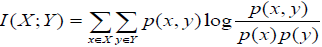
In order to assert if the four frequency signals contain common information about a particular seismic event, we need to investigate the relationship among them in terms of an information-theoretic criterion, such as the mutual information measure. For two discrete random variables, X and Y, the mutual information, I(X;Y) is given as
 (1)
(1)
With p(x,y) the joint probability distribution of X and Y and p(x), p(y) the marginal probability distributions of X and Y, respectively, these probability distributions are estimated through histogram methods [28]. Intuitively, mutual information measures how much information is shared between two random variables. A zero mutual information value means that X and Y are independent and knowing one variable provides zero knowledge about the other. The upper bound of the mutual information measure of X with another random variable is I(X;X) = H(X), with H(X) the entropy of random variable X. These last two properties can be easily verified by the equation I (X;Y) = H(X ) − H(X | Y ) .Applied to signal comparisons, a nonzero mutual information value means that the two signals share information. Furthermore, a high mutual information value means that the common information content of the two signals is high as well. In our scenario, we expect to have high mutual information between channels that are close in frequency since any particular time event should “spill over” to adjacent frequencies.
SVM features extraction
As mentioned in section 2.1, the EM data processed by the longmemory analysis method are labeled as fBm if 1 < b < 3 and r2 > 0.95, otherwise they are labeled as non-fBm. A two-class segmentation thus arises, which can be elegantly handled by a supervised classifier. Among the several classifiers, the SVM classifier is selected for its simplicity and the fact that no prior information or assumptions on the treated EM data is required. In its most basic form, SVM attempts to separate already labelled data via a hyperplane into two regions (classes) such that the gap between them is maximized, i.e., the point of class A closest to the hyperplane and the point of class B closest to the hyperplane are as far apart as possible. The data can also be mapped onto another, higher dimensional, space via a kernel function in case they are not linearly separable in the existing space.
The EM segments are typically long, which means that the SVM will have to process very long vectors during its training phase, i.e., during the derivation of the separating hyperplane. For this reason, it is wise to reduce the segments length by deriving features of much shorter length but of high information content. It is also desirable to select a computationally fast and simple features extraction scheme as the main benefit of the SVM classifier is the computational speed when compared to more complex methods such as the power-law wavelet method. Since we have full information on the algorithm of the separating process that leads to the two classes, i.e., the power-law wavelet analysis method, we attempt to follow the same or nearly the same mathematical steps with this method albeit with comparatively lower computational cost. Therefore, instead of the CWT, used in the power-law wavelet method, we employ the Fast Fourier Transform (FFT) which is among the fastest, computationally, transforms and specifically much faster than the CWT. Since the power-law wavelet method operates on the power spectrum, we also take the square magnitude of the FFT coefficients, after they have their mean removed and have been multiplied by a window function, to derive a crude estimate of the power spectrum. In order to reduce the features length and speed up the SVM computations later, we retain only half of the power spectrum coefficients (because of the FFT symmetry) and downsample by a factor of 8.
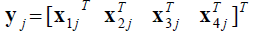
Applied to our scenario, the 1024 samples of the jth EM data segment of frequency channel i (i = 1, 2, 3, 4), enter the FFT to produce 1024 spectral coefficients. The lower 512 of them are retained and after downsampling by a factor of 8, we are left with the feature vector Xij of the jth EM segment of frequency channel i with length equal to 64 coefficients. Finally, the jth feature hypervector, which incorporates the features from all four frequency channels is given as,
 (1)
(1)
Notice that the length of hypervector yj is four times the length of vector Xij, i.e., equal to 256 coefficients. This is much smaller than the total length of four EM segments of 1024 samples each. This whole feature calculation process emulates the power-law wavelet analysis algorithm in a more simple and, possibly, less accurate way but much faster computationally. The feature hypervectors y is used during the training and testing phase of the SVM classifier. The criteria for separating these features into classes are analysed next.
SVM class separation via long-memory analysis
The SVM classification algorithm, being a supervised learning method, requires class-labelling of the hypervectors that are used for initially training the classifier. Our goal is to find a reliable criterion to label the EM segments whose features are used for training the SVM classifier. For our scenario, we need two classes. Class I consists of EM segments that are deemed as significant or of some earthquake precursory value. Class II consists of EM segments that are deemed as insignificant or of no earthquake precursory value. Apparently, Class II EM segments are the complement of Class I segments. If all four parallel segments starting at a particular time instance yield successive fBm behaviour (r2 > 0.95 and 1 < b < 3), then the particular time instance is declared as significant or of some precursory value. If at least one of the four parallel segments yields non-fBm or not successive fBm behaviour (case with b∉(1 , 3) and case with r,2 > 0.95 and 1 < b < 3), then the particular time instance is declared as insignificant or of no precursory value. The above annotation can be extended to the corresponding hypervectors and thus we define a
• Class I hypervector if all four channel segments are successive fBm (r2 > 0.95 and 1 < b < 3)
Class II hypervector if at least one channel segment is nonsuccessive fBm or non-fBm (case with r2 > 0.95 and 1 < b < 3 or case withb∉(1 , 3) ).
The aforementioned hypervectors, along with their class annotation, are used as training data for the SVM classifier in order to derive its training parameters. The algorithmic procedure is presented in the form of a flow chart in Figure 1.

Figure 1: Algorithmic flow chart.
In the testing phase, the SVM classifies the testing data according to the stored training parameters. For a specific kernel function K( xi xj)=< φ(xi),φ(xj)> and mapping φ(â�?�?) of the feature vector x to a higher dimensional feature space, the decision process for classifying the testing data into Class I or Class II is given by sgn(wTφ (x) + c) , with sgn(â�?�?) the sign function and w, c part of the training parameters. The important point here is that once the training of the SVM is complete, i.e. the training parameters are derived; the decision process is very fast computationally. It is given by the sign of the inner product of two vectors, w and φ (X), after having been added to the constant c. In comparison, the original method of identifying Class I segments by applying the power-law wavelet method on all four channels incurs a much higher computational cost.
Implementation and Results
The algorithm described above is implemented for the scenario of EM data monitoring prior to earthquakes in Greece. By utilizing an extensive network of EM monitoring stations [26], we explore 20 earthquakes of magnitude ML ≥ 3.4 in a three-month time period, starting on 29/01/2011 and ending on 28/04/2011, located inside a radius of 150 km around the EM measurement station Neapoli Crete. Two of these earthquakes are of magnitude larger than ML = 5. The measurements consist of four EM data sequences corresponding to 3 kHz, 10 kHz, 41 MHz and 46 MHz radiations, respectively, with a sampling frequency of 1 Hz. This amounts to a length of approximately 7.8×10⁶ samples for each channel in a 90-day observation window. In our implemented scenario, we assume that we are continuously searching for anomalies in the EM readings without knowing the time of occurrence of the earthquake events. Fractal analysis through the described algorithms is done on a regular basis, e.g., at the end of each monitored day. Real time processing is more difficult, as long-memory analysis methods operate on successive, fixed length segments (e.g. 1024 samples), advancing one sample ahead each time i.e. the sliding window step is one sample. With these parameters, the analysis captures very fine EM variations in time at the expense of high computational cost as any given fractal analysis window almost completely overlaps the preceding one. Given the same window length and step size, and once the SVM training is complete, the SVM classification task can be performed more rapidly and real time processing is less computationally demanding.
The four EM recordings, corresponding to the four different EM radiation frequencies and spanning the 90-day period, are shown in Figure 2. Two major earthquakes occurred on 28/02/2011 (ML = 5.2) and 01/04/2011(ML = 6.2), corresponding to horizontal positions 2.6×10⁶ and 5.4×10⁶ in all subfigures of Figure 2, respectively. Thirteen other earthquakes of magnitude (ML = 3.5) up to (ML = 4.2) also occurred in the same time period. The area of observation is a circular area of radius 150 km centered on the Neapoli station in Crete.

Figure 2: Collective EM measurements of the 90-day time period (29/01/2011-28/04/2011) at Neapoli station for the data channels at: (a) 3 kHz, (b) 10 kHz, (c) 41 MHz and (d) 46 MHz, EM radiation.
Figure 3 presents the results of the power-law wavelet method applied on the EM sequences of Figure 2. It can be observed that all subplots present several segments with the square of the Spearman correlation coefficient above the critical value of 0.95, i.e., the fit to the power-law were excellent. This is a strong indicator of the fractal character of the underlying processes and structures [10,11]. This suggests that the underlying dynamics are governed by a positive feedback mechanism and that external influences tend to lead the system out of equilibrium [6,10,16]. Hence, the system acquires a self-regulating character and, to a great extent, the property of irreversibility, one of the important components of prediction reliability [6,10,16]. Under this perspective, the high power-law beta-value parts of Figure 3 imply long-range temporal correlations, i.e., strong system memory. Thus, each value correlates not only to its most recent value but also to its long-term history in a scale-invariant, fractal manner [6,10,16]. The history of this system defines its future (non-Markovian behaviour) [6,10,16]. From another viewpoint, the non-fBm parts (-1 < b < 1) are associated with “flicker noise” - 1/f behaviour which is a reflection of the fact that the final output of fracture is affected by many processes that act almost randomly on different time scales [3,4,6,10,16]. The above-mentioned fBm results are in good agreement with the relevant prediction based on the hypothesis that the evolution of the Earth’s crust towards the general failure may take place as a self-organized critical (SOC) phenomenon in a seismological sense [3,4,6,10,16]. All these are compatible with the last stage of earthquake generation [3,4,6,10,16]. Moreover, the high b-exponent values are indicative of candidate precursory activities. Indeed, the background noise, as being qualitatively analogous to the fGn-1/ f n ,n ï¦≅1 class, exhibits b-values between 0 and 1 [3,4,6,10,16]. On the contrary, electromagnetic precursory signals, being compatible with the fBm model, present b-values between 1 and 3 [3,4,6,10,16]. The latter fact indicates that the high value power-law beta parts of Figure 3 are compatible with a successive fBm model, which is consistent with the slip of two self-affine fractional Brownian surfaces during the generation of earthquakes [3,4,6,10,16]. Noticeable, is that the above behaviour is differentiated within the investigated 90-day EM recordings probably due to the differences in the magnitude, depth and distance from the recording station, as well as due to different sensitivity [17] of the recording station in reference to the occurrence area of the investigated earthquakes.

Figure 3: Estimation of spectral exponent b based on the power-law wavelet analysis method for the sequences of Fig.2 for the data channels at (a) 3 kHz, (b) 10 kHz, (c) 41 MHz and (d) 46 MHz. Blue points indicate successive fBm segments while red points indicate non-fBm or not successive fBm segments.
Up to this point, the four channels have been processed independently, each one of them producing different decisions on which time segments are critical, i.e., successive fBm. It is important to note that these four data channels monitor the same time events, albeit at different frequencies. Consequently, a seismic anomaly –if it is indeed critical- could manifest simultaneously over a range of frequencies at some degree. The reverse is cast as a stronger condition, i.e., EM anomalies appearing simultaneously in multiple frequency channels must correspond to a time instance of pre-seismic activity. In other words, we do not claim that all pre-seismic events of precursory value should appear in more than one EM frequencies but we claim that the reverse must be true, i.e., critical EM segments appearing simultaneously on many frequency channels are a very strong indicator of precursory seismic activity. Therefore, an intuitive way to decide if a particular time instance is of precursory value is to check whether fBm behaviour is present on all four channel segments corresponding to (i.e. starting at) that particular time instance.
In order to reinforce this logic, we attempt to show that there is dependence among the different channels that are close in frequency with that dependence diminishing for channel frequencies further apart. More specifically, we investigate the fractal behaviour of each channel through the b sequences of Figure 3 and seek for any similarities across different channels. The reasoning behind this is that if the fractal behaviour in each frequency channel does not vary randomly but is affected by an underlying seismic process, then there should be similarities in their b-patterns across various channels, with the similarities becoming stronger for channel frequencies that are close to each other.
Figure 4 presents these similarities in terms of the mutual information between b-sequences for various pairs of the four frequency channels of Figure 3. For each pair of frequency channels, an orthogonal window of length N+1 multiplies the b-sequence of the first channel and another, identical, window multiplies the b-sequence of the second channel. Assuming that the two windows start at sample N1 and N2, respectively, the mutual information between the two windowed b-sequences is computed, I[b1(N1,N1+N:)b2(N2,N2+N)],where b2(N2,N2+N) is the b-sequence of channel 1, starting at sample N1 and ending at sample N1+N, and b2(N2,N2+N) is the b-sequence of channel 2, starting at sample N2 and ending at sample N2+N. The two windows slide relative to each and the mutual information is computed for various values of N1 and N2. The results of this process for N = 1E6 samples are depicted for various pairs of frequency channels in the subfigures of Figure 4. Note that for relative sliding N1-N2 = 0, the two b-sequences are time-aligned, i.e., they correspond to exactly the same time period since the lag of the one sequence relative to the other is zero. In all subfigures, the b-sequence of channel 2 stays fixed, starting at sample N2 = 4E6 (i.e., around the center of the 90-day set as seen in Figure 3), while the b-sequence of channel 1 shifts forward or backward in time by varying the value of N1. For N1-N2 = ±1E6 samples, the two b-sequences do not overlap at all.

Figure 4: Mutual information between windowed and shifted b-sequences of (a) 3 kHz and 10 kHz channels, (b) 41 MHz and 46 MHz channels, (c) 3 kHz and 41 MHz channels and (d) 10 kHz and 46 MHz channels. The b-sequence of channel 2 is fixed, starting at N2=4E6 samples, while the window of channel 1 sequence slides forward or backward by N1-N2 samples.
Figures 4a and 4b show a main peak at N1-N2 = 0, i.e., when the b-sequences are time-aligned. The same does not apply for Figures 4c and 4d for which no maximum appears when the two sequences have zero lag between them. This means that for channel frequencies that are close to each other, the b-sequences share maximum common information when they correspond to the same time period, i.e., when their relative lag is zero. This above is true for other values of N2 as well, ranging from the beginning to the end of the 90-day period. Conversely, the b-sequences of channels with frequencies that are far part (e.g. 10 kHz and 46 MHz) exhibit mutual information that varies randomly with the lag N1-N2 and the same holds for other pairs with large frequency separation such as pairs 3 kHz-46 MHz and 10 kHz - 41 MHz.
Now that we have established that nearby frequency channels share common information, we attempt to fuse the independently taken decisions on successive fBm/not successive fBm of all four channels into a single decision. An intuitive way to visualize the decisions on successive fBm vs not successive fBm of the powerlaw wavelet analysis method for each channel is to model them as an On-Off process. This is shown in Figure 5 for the channel with frequency 41MHz. Starting from the whole b-sequence of the channel, we assign a value of 1 if we have successive fBm behaviour (r2 > 0.95 and 1 < b < 3) and we assign a value of zero otherwise. The result is a sequence of successive fBm segment locations (more specifically, locations of the first sample of each segment). Note that the positions of the successive fBm segments in Figure 5 match exactly the positions of the successive fBm b-values of Figure 3c (blue points).

Figure 5: Decision sequence on successive fBm segments of a single channel (41 MHz) modelled as an On-Off process. Successive fBm segments are assigned a value of 1 and all the remaining segments are assigned a value of 0.
The remaining three channels produce their own On-Off decision sequences. As explained in section 2.5, a straightforward way to combine these four decision sequences spanning the 90-day period is to take their intersection regarding the occurrence of successive fBm segments (1-values). Specifically, a time instance is declared critical if successive fBm segments are simultaneously detected in all four channels. This is shown in Figure 6, along with the 20 earthquake occurrences during the 90-day observation period. Note that, as the data sampling frequency is 1Hz and each new segment moves 1 sample (or 1 sec) ahead relative to the previous segment, the segment index axis is identical to a time axis in sec marking the start of each segment. The earthquake sequence, shown in Figure 7, has been acquired by the National Observatory of Athens (NOA) - Institute of Geodynamics BBNET database of seismic events (http://bbnet.gein.noa. gr/HL/database). Note that, generally, even in short-term prediction there is no one-to-one correspondence between abnormalities in the recordings and the seismic activity [29-31]. Nevertheless, we can make three very significant remarks on Figure 6:

Figure 6: Combined, four-channel On-Off decision sequence on critical segments plotted against the actual 20 earthquakes sequence of the 90-day period. Notice that from time 0 sec to around 1.5E6 sec, the absence of critical segments detection is in agreement with the absence of earthquake occurrences.

Figure 7: The earthquake magnitude sequence during the 90-day period for the area around Neapoli station as reported by NOA.
1. During the 17-days period from 0 sec to around 1.5E6 sec, the absence of earthquakes is in agreement with the absence of critical segments detection. This means that the four-channel fBm detection scheme does not produce any false alarms during periods of no seismicity. The same claim holds for the time period from approximately 5.5E6 sec to 6.1E6 sec and the time period from approximately 7.3E6 sec to 7.8E6 sec.
2. During the period from approximately 3.5E6 sec to 4.5E6 sec there are no earthquake occurrences but there are two distinct points for which four-channel fBm detection occurs, i.e. we have two false alarm areas of short duration. We have to note, though, that under the four-channel combined output the number of false alarms is definitely lower than the case of single-channel fBm detection. The reason for this is that the critical segments decision based on four-channel fBm detection is the intersection of four, single-channel, decisions. Therefore, the set of detected critical segments -including the falsely declared as such- under the four-channel scheme will be in practice a subset of any of the single-channel sets (in theory it could be at most equal). More simply, the number of false alarms when the four channels are combined is reduced as compared to the case of single-channel fBm detection. This can be easily verified by observing Figure 5, where the number of successive fBm segments is larger when compared to that of Figure 6.
3. It can easily be observed from Figure 6 that four-channel fBm occurences happen in the near vicinity of earthquake occurrences, e.g., at sample locations from (approximately) 5E6 to 5.5E6. More specifically, four-channel fBm detection happens within a maximum time period of three days (approximately 2.6E5 samples) before or after an earthquake.
An example of a feature hypervector y, used for SVM classification, is shown in Figure 8. The original four channel-segment length is 4096 EM measurements, leading to a feature hypervector consisting of 256 FFT (squared) coefficients. Notice the concatenation of four feature vectors x of length 64, each one corresponding to one of the four channels, as explained in section 2.4.

Figure 8: Typical feature hyper-vector extracted from a 4096-long segment consisting of four EM segments of 1024 samples each.
The SVM classification results are presented and analysed for the 90- day period under investigation. The LIBSVM library [32] is employed in order to implement the SVM task. The EM measurement sequence of each earthquake is divided into training and testing data. The readings corresponding to the first 30 days of the 90-day monitoring period are used as training data for the computation of the SVM parameters. The remaining EM readings, corresponding to the next 60 days of the 90- day monitoring period, are allocated for testing and evaluating the SVM classifier. Table 1 describes the training and testing sets, in terms of number of segments. It is expected that the number of Class II segments will be much higher than the number of Class I segments during the 90- day period. In order to have balanced training data, subsampling of the Class II segments in the time domain is employed such that the number of training segments of Class I and II is the same. More specifically, the training set is created by picking every 2000th Class II segment in the time domain and all Class I segments, resulting in 1006 training segments for each of the two classes. The SVM parameters set is finetuned by attempting to maximize the overall accuracy of the classifier, given by

| Recording Period | Training Set 29/01/2011-27/02/2011 (number of segments) |
Testing Set 28/02/2011-28/04/2011 (number of segments) |
||
|---|---|---|---|---|
| Class I | Class II | Class I | Class II | |
| 1006 | 1006 | 5239 | 5117381 | |
Table 1: Training and testing sets for SVM classification.
After a coarse grid parameter search, a SVM kernel function that classifies the testing data with high overall accuracy is found to be an inhomogeneous polynomial of degree four, given as K(xi,xj)=(γxixj+r)4 with γ = 1/140 and r = 10. This kernel is used throughout the classification experiments. The individual class accuracy is given as

The classification results are shown in Table 2. An overall accuracy rate of more than 86% is attained. It is noted that the SVM parameters set is fine-tuned towards equal accuracies for Class I and Class II segments but if more accuracy is required for, e.g., Class II at the expense of Class I accuracy we can fine-tune the SVM classifier parameters towards that end. Since the Class II testing segments are much more than the Class I testing segments, raising the Class II accuracy would raise the total accuracy as well which in our tests reached rates above 97%. In addition, the number of insignificant, Class II, segments that are falsely declared as significant, i.e., the number of false alarms, would decrease. However, we would detect fewer critical, Class I, segments which are significant for predicting earthquake occurrences. Notice that since this is a binary classifier, the accuracy rate of Class I is identical to the sensitivity rate while the accuracy rate of Class II is identical to the specificity rate. It is important to note that the classifier performed very well in classifying Class I segments even though there are very scarce (only 1006 segments for training). Adding to the scarcity of Class I segments, the variability of the Class I training set is quite low as critical segments are usually consecutive in time and differ from their adjacent ones by only one sample. More specifically, as the analysis window for the EM data progresses one sample each time, consecutive Class I segments are virtually the same, thus inhibiting the SVM’s performance.
| Recording Period | Accuracy Class I (sensitivity) % | Accuracy Class II (specificity) % | Overall Accuracy % |
|---|---|---|---|
| 28/02/2011-28/04/2011 | 86.4 (4526/5239) | 86.3 (4415681/5117381) |
86.3 (4420207/5122620) |
Table 2: SVM classification results.
Conclusions
This paper presented a multichannel, multi frequency approach on the analysis of EM data for precursory signs of earthquake occurrences. A period of 90 days, including 20 earthquakes of magnitude equal or larger than ML = 3.4, was studied. The contribution of this work can be summarized as follows:
1) The results of the power-law wavelet analysis, running on four parallel channels, were presented. Multiple fBm instances were identified in each channel, which are considered to be of significant precursory value.
2) In order to increase the reliability and accuracy of the fBm detection process, the fBm detection results of all four channels were combined to derive a single decision sequence for each time instance and declare it as critical or non-critical.
3) Results on information-theoretic similarities between adjacent – in frequency- channels showed that the multichannel detection strategy is meaningful and that significant anomalies and critical fluctuations do manifest in a range of frequencies, as it is naturally expected.
4) The four-channel detection sequence for the 90-day period was juxtaposed against the 20 main earthquakes of the same period. The results of the comparison are promising, as critical segments detection happened mostly in the near vicinity of earthquakes while there were very few false alarms, i.e. critical segments detection in periods when there was no earthquake occurrence. There was also a period of around 17 days (1.5E6 samples), in the beginning of the 90-day period, in which no earthquakes occurred and also no critical segments detection was reported. These findings are proof of the superiority of multichannel critical segments detection over the single-channel case.
5) Results on SVM classification showed that the EM data separation into significant and insignificant parts, performed using fourchannel power-law wavelet analysis, is also reproducible by the SVM classifier operating on reduced features of the original EM data. The main criterion for constructing the features was to emulate the power-law wavelet analysis, albeit at a higher computational speed so that the SVM can operate in real-time. The SVM accuracy attained was at least 86% with the advantage of low computational cost.
References
- Varotsos P, Alexopoulos K (1984) Physical properties of the variations of the electric field of the earth preceding earthquakes, I. Tectonophysics 110: 73-98.
- Varotsos P, Alexopoulos K (1984) Physical properties of the variations of the electric field of the earth preceding earthquakes, II, determination of epicenter and magnitude. Tectonophysics 110: 99-125.
- Smirnova N, Hayakawa M, Gotoh K (2004) Precursory behaviour of fractal characteristics of the ULF electromagnetic fields in seismic active zones before strong earthquakes. PhysChem Earth 29: 445–451.
- Smirnova, N, Hayakawa M (2007) Fractal characteristics of the ground-observed ULF emissions in relation to geomagnetic and seismic activities. J Atmos Sol-TerrPhys 69: 1833–1841.
- Hayakawa M, Hobara Y (2010) Current status of seismo-electromagnetics for short-term earthquake prediction. Geomat. Nat Haz.Risk 1: 115-155.
- Eftaxias K (2010) Footprints of non-extensive Tsallis statistics, self-affinity and universality in the preparation of the L'Aquila earthquake hidden in a pre-seismic EM emission. Physica A 389: 133-140.
- Varotsos P, Sarlis N, Skordas E (2011) Scale-specific order parameter fluctuations of seismicity in natural time before main shocks. EPL 96 :59002-p1/59002-p6.
- Kapiris P, Eftaxias K, Nomikos K, Polygiannakis J, Dologlou E, et al. (2003) Evolving towards a critical point: A possible electromagnetic way in which the critical regime is reached as the rupture approaches. Nonlinear Process Geophys 10: 511–524.
- Eftaxias K, Contoyiannis Y, Balasis G, Karamanos K, Kopanas J, et al. (2008) Evidence of fractional-Brownian-motion-type asperity model for earthquake generation in candidate pre-seismic electromagnetic emissions. NHESS 8: 657-669.
- Eftaxias K, Athanasopoulou L, Balasis G, Kalimeri M, Nikolopoulos S, et al. (2009) Unfolding the procedure of characterizing recorded ultra low frequency, kHz and MHz electromagnetic anomalies prior to the L’Aquila earthquake as pre-seismic ones – Part 1. NHESS 9: 1953-1971.
- Eftaxias K, Balasis G, Contoyiannis Y, Papadimitriou C, Kalimeri M, et al.(2010) Unfolding the procedure of characterizing recorded ultra low frequency, kHZ and MHz electromagnetic anomalies prior to the L’Aquila earthquake as pre-seismic ones - Part 2. NHESS 10: 275–294.
- Minadakis G, Potirakis S, Nomicos C, Eftaxias K (2012) Linking electromagnetic precursors with earthquake dynamics: An approach based on non-extensive fragment and self-affine asperity models. Physica A 391: 2232–2244.
- Potirakis S, Minadakis G, Eftaxias K (2012) Analysis of electromagnetic pre-seismic emissions using Fisher information and Tsallis entropy. Physica A 391: 300-306.
- Kapiris P, Polygiannakis J, Peratzakis A, Nomicos K, Eftaxias K (2002) VHF-electromagnetic evidence of the underlying pre-seismic critical stage. Earth Planets Space 54: 1237–1246.
- Stavrakas I, Clarke M, Koulouras G, Stavrakakis G, Nomicos C (2007) Study of directivity effect on electromagnetic emissions in the HF band as earthquake precursors: Preliminary results on field observations. Tectonophysics 431: 263–271.
- Petraki E, Nikolopoulos D, Fotopoulos A, Panagiotaras D, Koulouras G, et al. (2013) Self-organised critical features in soil radon and MHz electromagnetic disturbances: Results from environmental monitoring in Greece. Appl. Radiat. Isot. 72: 39–53.
- Petraki E, Nikolopoulos D, Chaldeos Y, Coulouras G, Nomicos C, et al. (2014) Fractal evolution of MHz electromagnetic signals prior to earthquakes: results collected in Greece during 2009.Geomat. Nat. Haz. Risk 7: 550-564.
- Yonaiguchi N, Ida Y, Hayakawa M, Masuda S (2007) Fractal analysis for VHF electromagnetic noises and the identification of preseismic signature of an earthquake. J Atmos Sol-TerrPhys 69: 1825-1832.
- Kalimeri M, Papadimitriou C, Balasis G, Eftaxias K (2008) Dynamical complexity detection in pre-seismic emissions using non-additive Tsallis entropy. Physica A 387: 1161-1172.
- Eftaxias K, Panin V, Deryugin Y (2007) Evolution-EM signals before earthquakes in terms of meso-mechanics and complexity. Tectonophysics 431: 273–300.
- Cicerone R, Ebel J, Britton J (2009) A systematic compilation of earthquake precursors. Tectonophysics 476: 371-396.
- Nikolopoulos D, Petraki E, Marousaki A, Potirakis S, Koulouras G, et al. (2012) Environmental monitoring of radon in soil during a very seismically active period occurred in South West Greece. JEM 14: 564-578.
- Nikolopoulos D, Petraki E, Vogiannis E, Chaldeos Y, Giannakopoulos P, et al. (2014) Traces of self-organisation and long-range memory in variations of environmental radon in soil: Comparative results from monitoring in Lesvos Island and Ileia (Greece). JRadioanalNuclChem 299: 203-219.
- Cantzos D, Nikolopoulos D, Petraki E, Nomicos C, Yannakopoulos PH, et al. (2015) Identifying long-memory trends in pre-seismic mhz disturbances through support vector machines.J Earth SciClim Change 6: 1-9.
- Vapnik V (1998) Statistical learning theory, John Wiley & sons, New York.
- Vallianatos F, Nomikos K (1998) Seismogenicradioemissions as earthquake precursors in Greece. PhysChem Earth 23: 953-957.
- Torrence C, Compo GP (1998) A practical guide to wavelet analysis. Bull Am Met Soc 79: 61–78.
- ModdemeijerR (1989) On estimation of entropy and mutual information of continuous distributions. Signal Processing 16: 233-246.
- Petraki E, Nikolopoulos D, Nomicos C, Stonham J, Cantzos D, et al. (2015) Electromagnetic pre-earthquake precursors: Mechanisms, data and models-A review. J Earth SciClim Change 6: 1-11.
- Nikolopoulos D, Petraki E, Marousaki A, Potirakis S, Koulouras G, et al. (2012) Environmental monitoring of radon in soil during a very seismically active period occurred in South West Greece. J Environ Monitor 14: 564-578.
- Eftaxias K, Balasis G, Contoyiannis Y, Papadimitriou C, Kalimeri M, et al. (2010) Unfolding the procedure of characterizing recorded ultra low frequency, kHZ and MHz electromagnetic anomalies prior to the L’Aquila earthquake as pre-seismic ones - Part 2. NHESS 10: 275–294.
- Chang CC, Lin CJ (2011) LIBSVM: A library for support vector machines ACM Transactions on Intelligent Systems and Technology 2: 1-27.
Relevant Topics
- Atmosphere
- Atmospheric Chemistry
- Atmospheric inversions
- Biosphere
- Chemical Oceanography
- Climate Modeling
- Crystallography
- Disaster Science
- Earth Science
- Ecology
- Environmental Degradation
- Gemology
- Geochemistry
- Geochronology
- Geomicrobiology
- Geomorphology
- Geosciences
- Geostatistics
- Glaciology
- Microplastic Pollution
- Mineralogy
- Soil Erosion and Land Degradation
Recommended Journals
Article Tools
Article Usage
- Total views: 12713
- [From(publication date):
August-2016 - Apr 01, 2025] - Breakdown by view type
- HTML page views : 11795
- PDF downloads : 918