Research Article Open Access
Forecasting Copadichromis (Utaka) Production for Lake Malaŵi, Nkhatabay Fishery- A Stochastic Model Approach
Zaindi I*, Singini W and Mzengereza KMzuzu University, Department of Fisheries science Private Bag 201, Mzuzu 2, Malawi
- *Corresponding Author:
- Zaindi I, Mzuzu
University, Department of Fisheries
science Private Bag 201
Mzuzu 2, Malawi
T el: +265 1 320 722
E-mail: izaindi@gmail.com
Received Date: October 07, 2015; Accepted Date: January 11, 2016; Published Date: January 21, 2016
Citation: Zaindi I, Singini W, Mzengereza K (2016) Forecasting Copadichromis (Utaka) Production for Lake Malawi, Nkhatabay Fishery- A Stochastic Model Approach. J Fisheries Livest Prod 4:162. doi:10.4172/2332-2608.1000162
Copyright: © 2016 Zaindi I, et al. This is an open-access article distributed under the terms of the Creative Commons Attribution License, which permits unrestricted use, distribution, and reproduction in any medium, provided the original author and source are credited.
Visit for more related articles at Journal of Fisheries & Livestock Production
Abstract
Due to the overexploitation of Chambo (Oreochromis species), other species such as Utaka (Copadichromis species) have become important part of Lake Malaŵi, Nkhatabay fishery. The shift to Copadichromis species has put the stocks on danger of being overexploited just as was the case with Chambo (Oreochromis species). The study was therefore conducted to forecast Copadichromis (Utaka) species yield for Lake Malaŵi Nkhatabay fishery from 2010 to 2019. The study was based on the data of fish catches during the years from 1976 to 2009. The study considered Autoregressive Integrated Moving Average (ARIMA) model to select the appropriate stochastic model for forecasting Copadichromis species yield. Maximum likelihood estimation (MLE) method was considered in estimating the parameters. Based on ARIMA (p, d, q) and its components Autocorrelation function (ACF), Partial autocorrelation (PACF), Normalized Bayesian Information Criterion (NBIC), Box – Ljung Q statistics and residuals estimated, ARIMA (1, 1, 1) was selected. Based on the chosen model, it could be predicted that the Copadichromis species yield would decrease from 424.9tons in 1976 to 174.13tons in 2019. As the study has shown that Copadichromisspecies production will decrease, stakeholders in the management of fisheries resources should use this study to make policies and formulate strategies that will sustain yield of Copadichromis species.
Keywords
Forecasting; ARIMA; NBIC; Lake Malawi: Nkhatabay Fishery; Copadichromis; Modelling; Production
Introduction
Fisheries and aquaculture make crucial contributions to the world’s wellbeing and prosperity. In the last five decades, world fish food supply has outpaced global population growth, and today fish constitutes an important source of nutritious food and animal protein for much of the world’s population [1]. In addition, the sector provides livelihoods and income, both directly and indirectly, for a significant share of the world’s population. World over, fisheries support about 560 million people which is approximately 8% of the world’s population and the number is growing [2]. Of about 34 million active fishers, more than 90% are small-scale operators [3]. Fish and fishery products are among the most traded food commodities worldwide, with trade volumes and values reaching new highs of US$125 billion in 2011 andexpected to carry on rising, with developing countries continuing to account for the bulk of world exports [1].
In Malawi , fishing is the traditional occupation for most of the rural communities along the lakes and rivers. With 20% of Malawi ’s surface area covered by water, fish is one of the commonest source of animal protein and a major source of income. Over 70% of the animal protein consumed comes from fish and fisheries contribute about 4% to Gross domestic product [3]. Over 55000 fishers directly earn their income from fishing operations and nearly 300000people are involved in various fisheries related activities in Malawi (Fisheries Department, 2004).The fisheries sector in Malawi has two main groups; small scale/ artisanal fisheries and large scale fisheries. The artisanal fisheries contribute 85% of the total fish catch and constitute 90% of the fishers [4]. These fishermen are concentrated around all major water bodies of Malawinamely; lake Malawi , lake Malombe, lake Chiuta, lake Chirwa and the Shire river. Artisanal fisheries share the large part of Malawian fisheries. In Malawi, artisanal fisheries are open access, highly complex, scattered in all water bodies and mainly operate between 0-20m in Lake Malawi. The artisanal fisheries comprises of a wide range of fishingunits ranging from traditional fishing gears and craftssuch as fish traps and handlines operated from dugout canoes to relatively modern gears and crafts like the seine nets operated from planked boats powered by outboard motors and employ a lot of people. In this background, this study was conducted to forecast pattern of Copadichromis species yield in Lake Malawi, so as to help in formulating the needed strategies for sustainable management and conservation of the stock.
Materials and Methods
Modeling and forecasting have a long history of research. It was the major contribution of Yule which launched the notion of stochasticity in time series by postulating that every time series can be regarded as the realization of a stochastic process. Based on this idea, a number of time series methods have been proposed. Box and Jenkins [5] integrated the existing knowledge on time series. They introduced univariate models for time series which simply made systematic use of the information included in the observed values of time series. This offered an easy way to predict the future development of the variable. Moreover, these authors developed a coherent, versatile three-stage iterative cycle for time series identification, estimation, and verification. Several methods for identifying ARIMA models have been suggested by Box- Jenkins and others. Akaike discussed the stationary time series by an AR (p), where p is finite and bounded by the same integer. Moving Average (MA) models were used by Slutzky. Hannan and Quinn suggested obtaining the order of a time series model by minimizing the errors for pure AR models, and Hannan for ARMA models. While Mendelssohn used Box-Jenkins models to forecast fishery dynamics, Prajneshu and Venugopalan discussed various statistical modeling techniques viz., polynomial, ARIMA time series methodology and nonlinear mechanistic growth modeling approach for describing marine, inland as well as total fish production in India during the period 1950-51 to 1994-95. Stergiou et al. also evaluated the seasonal part of ARIMA and indicated that seasonal ARIMA(1,0,1), (0,1,2)12 models fitted and forecasted the monthly pelagic fish catches in Hellenic waters, the model provided low value of Bayesian information criteria (BIC), medium standard error and mean absolute percentage error. Seasonal ARIMA takes into account the seasonal component of the time series data. Chi-Lu and Su-Zan evaluated the efficiency of Box and Jenkins ARIMA model in the short-term forecasting of the fishery, using the time series of monthly catch and the monthly catch per unit effort (CPUE) of the South Atlantic albacore harvested by the Taiwanese long-line fishery from January 1968 to December 1993. The model provides a useful measure of the likely ranges of catch and CPUE for the management of albacore stock in the South Atlantic Ocean. Although ARIMA models have been widely used, there have been some critiques of the model. Critiques of the ARIMA regard such model to be very too simplistic, subjective, agnostic in nature. They find many disadvantage of ARIMA model as it neglects the inclusion of explanatory variables and conducts the forecasts only on past values of the dependent variable in combination with present and past moving average terms. For example, Kandananond [6] compared various forecasting methods for auto correlated time series. He compared artificial neural network (ANN), Support Vector Machine (SVM) and Autoregressive integrated moving average (ARIMA) models. He concluded that SVM and ANN were the best methods of forecasting since they included explanatory variables. Azad used ARIMA and exchange rate neural network (ERNN) models in forecasting Exchange Rates of Bangladesh. They have found that ERNN model shows better performance than ARIMA However, many empirical studies have been done regarding the effectiveness of ARIMA model in forecasting. Tsitsika et al. used univariate and multivariate ARIMA models to model and forecast the monthly pelagic production of fish species in the Mediterranean Sea during 1990-2005. Jai Sankar and Prabakaran [7] used ARIMA model to model and forecast milk production in Tamilnadu during 1978-2008. Sankar et al. [8] also used stochastic modeling for cattle production and forecast the yearly production of cattle in the Tamilnadu state during 1970-2010. Another related study was done by Iqbal et al. to forecast the production of wheat in Pakistan up to 2022 using last thirty years data of area and production on wheat for modeling purpose. In Malawi, fish catch forecasting has been neglected [9]. Few time series analysis studies has been done but none for Nkahatabay fishery. Singini et al. [6] used ARIMA to model and forecast Copadichromis species (Kambuzi) production in Malawi and also used ARIMA to model and forecast Oreochromis species (Chambo) production in Malawi using data from 1976 to 2011in 2013. Another Study was done by Lazaro and Jere (2013) who forecasted the status of commercial Chambo (Oreochromis species) fishery in Malawi from 2011 to 2020. ARIMA model involved four steps: Identification, estimation, diagnostic checking and forecasting. Model identification involved examining plots of the time series data to find if the variance was stable in the data. Model identification involved examining plots of the sample autocorrelograms and partial autocorrelograms and inferring from patterns observed in these functions the correct form of ARMA model to select. Gujarati (2004) pointed out that when the PACF has a cutoff at p while the ACF tails off, it gives an autoregressive of order p (AR (p)). If the ACF has a cutoff at q while the PACF tapers off, it gives a moving-average of order q (MA (q)). However, when both ACF and PACF tail off, it suggests the use of the autoregressive moving-average of order p and q (ARMA (p, q)).
Autoregressive process of order (p) is,
 (1)
(1)
Moving Average process of order (q) is,
 (2)
(2)
Autoregressive moving average: ARMA of order (p, q) is,
 (3)
(3)
The general form of ARIMA model of order (p, d, q) is
 (4)
(4)
Where Yt is the observation at time t, and φ, θ are coefficients and ε is an error term.
Model fitting consisted of finding the best possible estimates for the parameters of the tentatively identified models. In this stage, maximum likelihood estimation (MLE) method was considered to estimate the parameters. (MLE) method for estimation of ARIMA was applied in SPSS version 16.0. MLE runs an algorithm several times, using as the starting point the solution obtained in the previous iteration/run. Basically SPSS maximizes the value of a function by choosing the set of coefficient estimates that would maximize the function. Each time, it uses the estimates obtained in the previous iteration/run. In model diagnostics, various diagnostics such as the method of autocorrelation of the residuals and the Ljung-Box-Pierce statistic were used to check the adequacy of the identified models. If the model was found to be inappropriate, the process was returned back to model identification and cycle through the steps until, ideally, an acceptable model was found. Plots of autocorrelation and partial autocorrelation of the residuals were used to identify misspecification. For evaluating the adequacy of ARMA and ARIMA processes, various statistics like Correlogram of the residuals; Normalized Bayesian Information Criterion (BIC), R-square, Stationary R-square, Root Mean Square Error (RMSE), Mean Absolute Percentage Error (MAPE), Maximum Absolute Percentage Error (MaxAPE), Mean Absolute Error (MAE) and Maximum Absolute Error (MaxAE) were used. In this study data on fish catch in Lake Malawi, Nkhatabay fishery was generated based on programme called Catch Assessment Survey (CAS) from the Department of Fisheries Research Unit at Monkeybay, Government of Malawi from 1976 to 2009. The data were used to fit the ARIMA model to predict the future yield of Copadichromis species in Lake Malawi, Nkhatabay fishery.
Results and Discussion
Model identification
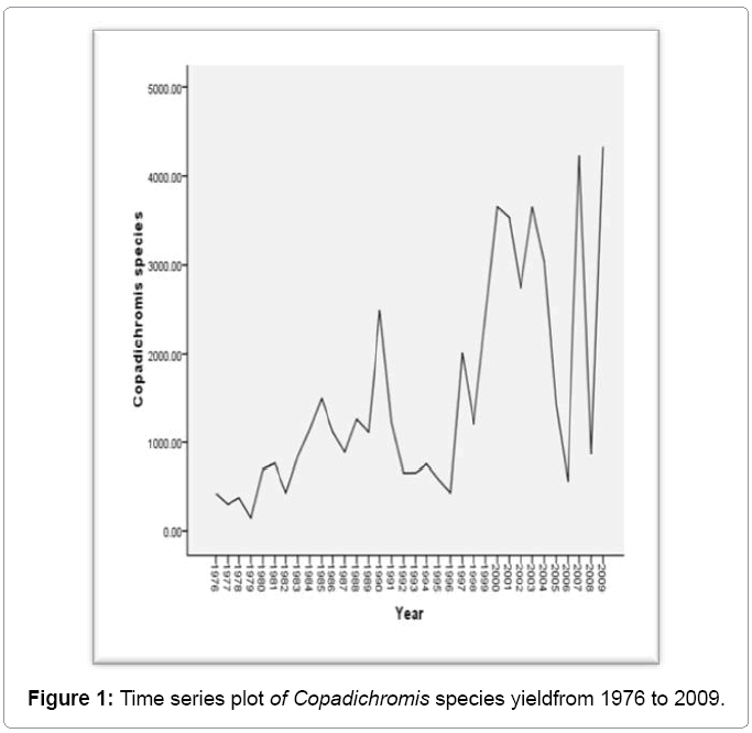
The first step in model identification was the preliminary analysis for examining stationarity of the data. ARIMA model was designed after assessing that transforming the variable under study was a stationary series. According to Sankar [7] the stationary series is the set of values that vary over time around a constant mean and constant variance and the most common method used to check the stationarity is through explaining the data by graph as shown in Figure 1 below:
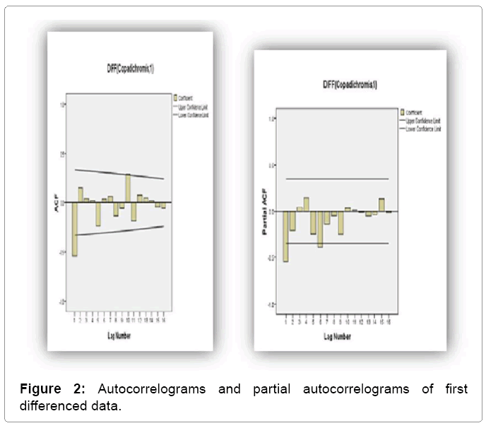
From the graph in Figure 1, it is apparent that the data is not stationary due to presence of trends in some sections throughout the 1976 to 2009 period. Zuur and Pierce [10] observed that most fisheries data is non-stationary. The problem of non-stationarity was over came through first order differencing of the data and stationary test were made on newly constructed series of the data. The process of making the series stationary agrees with Guti´errez-Estrada et al. [11] who showed that a good autoregressive model of order p (AR (p)) has to be stationary, and a good moving average model of order q (MA (q)) has to be invertible. Invertibility and stationarity will give a constant mean, variance, and covariance. Since the new series was stationary, the next step was to identify the values of p and q. For this, the autocorrelation and partial autocorrelation coefficients (ACF and PACF) of various orders of Yt were computed and represented in Figure 2 and Table 1.
| Lag | ACF | Std. Error Value | df | Sig | PACF | Std Error | |
|---|---|---|---|---|---|---|---|
| 1 | -0.544 | 0.166 | 10.675 | 1 | 0.001 | -0.544 | 0.174 |
| 2 | 0.149 | 0.164 | 11.502 | 2 | 0.003 | -0.208 | 0.174 |
| 3 | 0.043 | 0.161 | 11.573 | 3 | 0.009 | 0.041 | 0.174 |
| 4 | 0.021 | 0.158 | 11.591 | 4 | 0.021 | 0.146 | 0.174 |
| 5 | -0.24 | 0.156 | 13.962 | 5 | 0.016 | -0.243 | 0.174 |
| 6 | 0.04 | 0.153 | 14.029 | 6 | 0.029 | -0.389 | 0.174 |
| 7 | 0.067 | 0.15 | 14.229 | 7 | 0.047 | -0.142 | 0.174 |
| 8 | -0.133 | 0.147 | 15.049 | 8 | 0.058 | -0.049 | 0.174 |
| 9 | -0.057 | 0.144 | 15.203 | 9 | 0.086 | -0.248 | 0.174 |
| 10 | 0.289 | 0.141 | 19.394 | 10 | 0.036 | 0.035 | 0.174 |
| 11 | -0.187 | 0.138 | 21.239 | 11 | 0.031 | 0.011 | 0.174 |
| 12 | 0.078 | 0.135 | 21.578 | 12 | 0.043 | -0.012 | 0.174 |
| 13 | 0.05 | 0.132 | 21.72 | 13 | 0.06 | -0.052 | 0.174 |
| 14 | 0.018 | 0.128 | 21.741 | 14 | 0.084 | -0.038 | 0.174 |
| 15 | -0.046 | 0.125 | 21.876 | 15 | 0.111 | 0.136 | 0.174 |
| 16 | -0.056 | 0.121 | 22.086 | 16 | 0.14 | -0.013 | 0.174 |
Table 1: ACF and PACF for first order differenced scores of Copadichromis species.
The tentative ARIMA models are discussed with values differenced once (d=1). The value of p was found to be 1 and p ranged from 1 to 6. The model which had the minimum Normalized BIC was selected. The various ARIMA models and the corresponding Normalized BIC values are given in Table 2. The value of the Normalized BIC of the selected ARIMA was 14.530 and the most suitable model for Copadichromis is ARIMA (1, 1, 1), as this model had the lowest normalized BIC value. According to Czerwinski et al. [12] the best model should have adequate accuracy measures (RMSE, MAE) for it to have accurate forecasts and thus why the model was chosen since it had meet the requirements.
| Model | SR2 | R2 | RMSE | MAPE | MAX APE | MAE | MAX AE | NBIC |
|---|---|---|---|---|---|---|---|---|
| ARIM | 0.772 | 0.344 | 1092 | 1138 | 3251 | 740.9 | 3037 | 14.317 |
| A | 198 | 931 | 3.07 | 94 | 0.212 | |||
| (1,1,1) | 2 | |||||||
| ARIM | 0.772 | 0.345 | 1110 | 1152 | 3292 | 738.6 | 3030 | 14.459 |
| A | 876 | 955 | 2.29 | 49 | 0.304 | |||
| (1,1,2) | 5 | |||||||
| ARIM | 0.776 | 0.357 | 1121 | 2050 | 6138 | 743.6 | 3057 | 14.586 |
| A | 95 | 787 | 9.38 | 69 | 0.299 | |||
| (1,1,3) | 8 | |||||||
| ARIM | 0.779 | 0.364 | 1135 | 1789 | 5335 | 729.7 | 3002 | 14.72 |
| A | 659 | 744 | 3.03 | 88 | 0.126 | |||
| (1,1,4) | 4 | |||||||
| ARIM | 0.774 | 0.352 | 1169 | 1374 | 4013 | 721.2 | 3352 | 14.887 |
| A | 394 | 556 | 2.16 | 33 | 0.064 | |||
| (1,1,5) | 3 | |||||||
| ARIM | 0.835 | 0.525 | 1021 | 1667 | 4928 | 650.4 | 2216 | 14.725 |
| A | 742 | 686 | 4.97 | 99 | 0.327 | |||
| (1,1,6) | 3 |
Table 2: Model selection criteria.
Model estimation
After identifying the model the next step was to estimate the model. The coefficients parameters of the model were found to be statistically significant; a requirement for forecasting models. Czerwinski et al. [12] indicated that the Normalized BIC test reveals that the model with the least Normalized BIC is better in terms of forecasting performance than the one with a large Normalized BIC. Model parameters of the selected model were estimated using SPSS version 16.0 and the results of estimation are presented in Table 3.
| Model | Model | Coefficient | SE Coefficient | T value | P value |
|---|---|---|---|---|---|
| ARIMA | Constant | 2.237 | 12.496 | 0.179 | 0.859 |
| (1,1,1) | |||||
| AR | -0.634 | 0.175 | -3.615 | 0.001 | |
| MA | 0.991 | 1.341 | 0.739 | 0.466 |
Table 3: Final estimates of Copadichromis species ARIMA.
Diagnostic check
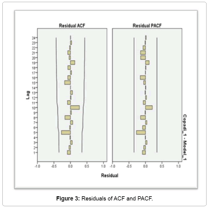
This involved checking the residuals of the model to see if they contained any systematic structure which still could be removed to improve the selected ARIMA. Diagnostic checking was achieved by examining the autocorrelations and partial autocorrelations of the residuals of various orders. Various autocorrelations up to 24 lags were computed and plotted as indicated in Figure 3. As the plots of ACF and PACF residuals indicate, none of autocorrelations was significantly different from zero at any reasonable level and were within 95% confidence interval. This proved that the selected ARIMA model was an appropriate model for forecasting Copadichromis species for Nkhatabay fishery. Therefore, the fitted ARIMA model for Copadichromis species production data was: 
Forecasting
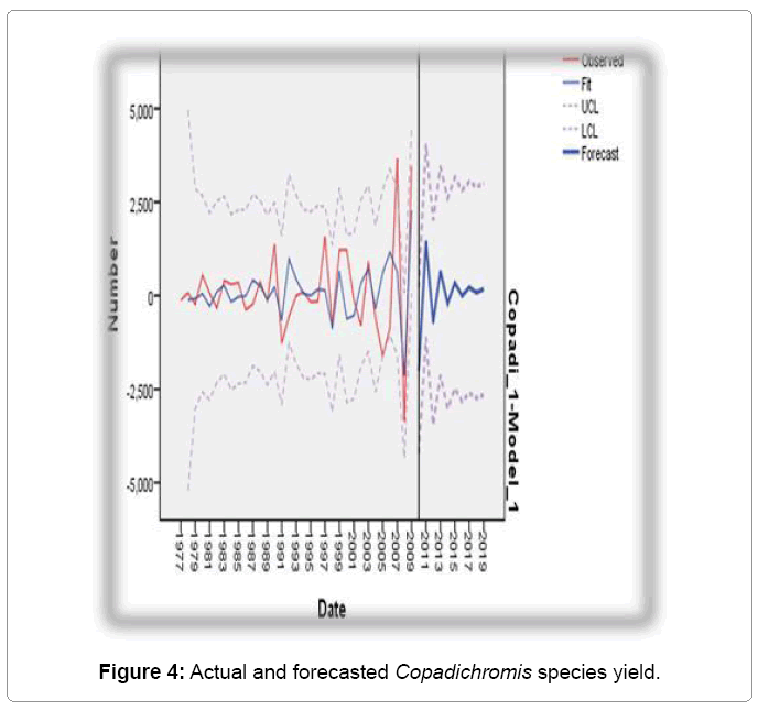
To assess the forecasting ability of the fitted ARIMA model, the measures of the sample period forecasts’ accuracy were computed. This measure also indicated that the forecasting inaccuracy was low. Table 4 shows the forecasted value of for Copadichromis species yield (with 95confidence limit). Czerwinski et al. [12] argued that a good model has a low forecasting error, therefore when the magnitude of the difference between the forecasted and actual values are low then the model has a good forecasting power and if the difference is high, then the model has a low forecasting power. This study noted that the magnitude of the difference between the forecasted and actual values were low for the selected model [13-20]. The noise residuals were combinations of both positive and negative errors which shows that, the model is not forecasting too low on the average or too high on the average. Having this positive behavior of the model, the model has outperformed as far as the forecasting power of the model is concerned. Figure 4 shows the actual and forecasted value of Copadichromis species yield with 95% confidence interval. From the forecast available from the fitted ARIMA model, it can be found that forecasted Copadichromis species yield would decrease from 424.9 tons in 1976 to 174.13 tons in 2019 [21-28].
| Year | Forecasted catch | 95% confidence bound |
|---|---|---|
| 2010 | -2002.78 | (-4216.93, 211.37) |
| 2011 | 1465.6 | (-1118.57, 4049.77) |
| 2012 | -727.99 | (-3468.61, 2012.64) |
| 2013 | 665.32 | (-2122.48, 3453.12) |
| 2014 | -213.7 | (-3028.30, 2600.91) |
| 2015 | 346.82 | (-2473.48, 3167.11) |
| 2016 | -4.62 | (-2830.24, 2821.00) |
| 2017 | 221.67 | (-2604.15, 3047.50) |
| 2018 | 81.97 | (-2745.07, 2909.01) |
| 2019 | 174.13 | (-2652.64, 3000.90) |
Table 4: Forecasted yield of Copadichromis species (in tons) for Lake Malaŵi, Nkhatabay fishery.
Conclusion
The most appropriate ARIMA model for Copadichromis species yield forecasting was found to be ARIMA (1, 1, 1). From the forecast available from the fitted ARIMA model, it can be found that forecasted Copadichromis species yield would decrease from 424.9 tons in 1976 to 174.13 tons in 2019. That is, using time series data from 1976 to 2009 on Copadichromis species yield, this study provides evidence on future Copadichromis species yield in Lake Malawi, Nkhatabay fishery, which can be considered for future policy making and formulating strategies for augmenting and sustaining Copadichromis species yield.
References
- FAO (2008) Malawi Fishery and AquacultureCountry Profile,Rome: Food and Agricultureorganisation of the United Nations (FAOUN).
- Eide A, Bavinck M, Raakjaer J (2011) Poverty Mosaics:Realities and Prospects In Small-Scale Fisheries. In: Jentoft S, Eide A (eds.) Avoiding poverty-Distributing wealth in fisheries.Dordrecht, London: Springer: 13-25.
- FAO (2004) The state of world fisheries andaquaculture, Rome: Food and AgricultureOrganisation of the United Nations.
- Kanyerere GZ, Namoto W, Mpoda O (2001) Analysis of Catch and Effort Data or the Fisheries of Nkhata Bay, Lake Malawi, 1976-1999,Lilongwe: 1-16
- Box GE, Jenkins GM (1970) Time SeriesAnalysis -Forecasting and Control.San Francisco:Holden-DayInc
- Singini W, Kaunda E, Kasulo V, Jere W (2012) Modelling and Forecasting Small Haplochromine Species (Kambuzi) Production in Malawi-A Stochastic Model Approach. International Journal of scientific & technology research 1: 69-73.
- Sankar J (2011) Forecasting Fish Product Export in Tamilnadu? A Stochastic Model Approach.Journal of Recent Research in Science and Technology 3: 104-108.
- Sankar J, Prabakaran R, Sethamarai K, Suresh S (2010) Stochastic Moddeling Approach for Cattle Production Forecasting. Journal of Modern Mathematics and Statistics 4: 53-57.
- SADC Secretariate (2009) Regional early warning system for food security; selected technical papers on methodology of food crop forecasting in SADC, Gaborone.
- Zuur A, Pierce G (2004) Common trends in northeast Atlantic squid time series. Journal of Sea Research 52: 57-72.
- Estradade GE, Pedro SJ, Luque EO, Calvo IP (2004) Comparison between Traditional Methods and Artificial Neural Networks for Ammonia Concentration Forecasting in an Eel (Anguilla Anguilla L.) Intensive Rearing System. AquatEng 31: 183-203.
- Czerwinski IA, Estrada JC, Hernandoc JAC (2007) Short-Term Forecasting of Halibut CPUE: Linear and Non-Linear Univariate Approaches. Fisheries Research 86: 120-128.
- Banda M, Kanyerere G, Rusuwa B (2003) Thechamborestoration strategic plan. In: Banda M, Jamu D, Njaya F, Makuwila M, Maluwa A (eds)The status of the chambo in Malawi: fisheries and biology,WorldFishCenter, Mangochi, Malawi. 1-7.
- Bazigos G (1972) The Improvement of theMalawianFisheries Statistical System. A report to the Integrated Project.
- Hampton J (2005) Changes in Abundance of Large Pelagic Predators in the Pacific Ocean:Nature.
- HilbornR, WaltersC (1992) Quantitative Fisheries Stock Assessment. Choice,Dynamics and Uncertainty. London 2: 177-178
- JamuD, ChimatiroS (2005) Sustainable agro-pisciculture in Malawi. In: Agriculture and Rural Development:Contributing to International Cooperation: 45-46.
- LazaroM, JereWWL (2013) The Status of the Commercial Chambo (Oreochromis Species) fishery in Malawi: A Time Series Approach. International Journal of Science and Technology3:1-6.
- MaunderM, PuntA (2004) Standardizing catch and effort data: a review of recent approaches.Fisheries Research 70: 141-159.
- MaunderM, Sibertb JR, Fonteneauc A, Hamptond J, Kleibere P, et al. (2006) Interpreting Catch Perunit effort Data to Assess the Status of Individual Stocks and Communities. ICES Journal of Marine science 63: 1373-1385.
- National Statistical Office(NSO) (2008) Population and Housing Census, Zomba: National Statistical Office, Government Print.
- NgwiraS (2012) Catch and effort analysis of small scale fishery of Nkhatabay district.
- Pierce G, Boyle P (2003) Empirical modeling of interannual trends in abundance of squid (Loligoforbesi) in Scottish waters. Fisheries Research59: 305-326.
- ShitanM, WeePJ, ChinL, SiewL (2008)Arima and integrated Arfima Models for Forecasting Annual Demersal and Peragic marine fish production in Malaysia. Malaysian Journal of mathematical sciences2: 41-54.
- TweddleD, AlimosoS, SodzapanjaG (1995) Analysis of catch and effort data for the fisheries of Nkhatabay Area, 1976-1987Goverment of Malawi, Fisheries.Bulletin.
- UNDP (2006) World Population prospects: The 2006 revision population database. New York: United Nations Population Division
- WalkerR (1976) Collection of Catch Assessment Data in Tropical Fisheries (Inland waters)Notes for Malawi Fisheries Deptuse.
- WHO (2006) Country Cooperations strategy at a glance Geneva: World Health Organisation.
Relevant Topics
- Acoustic Survey
- Animal Husbandry
- Aquaculture Developement
- Bioacoustics
- Biological Diversity
- Dropline
- Fisheries
- Fisheries Management
- Fishing Vessel
- Gillnet
- Jigging
- Livestock Nutrition
- Livestock Production
- Marine
- Marine Fish
- Maritime Policy
- Pelagic Fish
- Poultry
- Sustainable fishery
- Sustainable Fishing
- Trawling
Recommended Journals
Article Tools
Article Usage
- Total views: 11105
- [From(publication date):
March-2016 - Mar 29, 2025] - Breakdown by view type
- HTML page views : 10070
- PDF downloads : 1035
