Short Communication Open Access
Examination of Tectonic Activity Based on Knickpoint Distribution and Movement Potential of Faults in Khuzestan Province, South West Zagros, Iran
Rezvan Khavari*Behbahan branch of Islamic Azad University, Department of Geology, Behbahan, Iran
- *Corresponding Author:
- Rezvan Khavari
Behbahan branch of Islamic Azad University
Department of Geology, Behbahan, Iran
Tel: +986152870109
E-mail: Re_khavari@yahoo.com
Received date: November 23, 2016; Accepted date: February 10, 2017; Published date: February 17, 2017
Citation: Khavari R (2017) Examination of Tectonic Activity Based on Knickpoint Distribution and Movement Potential of Faults in Khuzestan Province, South West Zagros, Iran. J Marine Sci Res Dev 7:222. doi: 10.4172/2155-9910.1000222
Copyright: © 2017 Khavari R. This is an open-access article distributed under the terms of the Creative Commons Attribution License, which permits unrestricted use, distribution, and reproduction in any medium, provided the original author and source are credited.
Visit for more related articles at Journal of Marine Science: Research & Development
Abstract
Although the distribution of fluvial knickzones, as an important geomorphic feature in bedrock river morphology, has been studied by many investigators, the role of them in examination of tectonic activity has not been well investigated [1], specially based on its comparision with movement potential faults over a broad area. This study examines the tectonic activity of Khuzestan province, South West Zagros, by considering two different parameters: distribution of the fluvial knickzones along Mountain Rivers and evaluation of faults activity in the study area. A segment of a river long-profile that is steeper than adjacent segments is commonly referred to as a knickzone or a knickpoint if it is visibly steeper than the trend of the longitudinal profile. Knickzones are often observed along bedrock rivers and the most visible form is a waterfall. Knickzones are supposed to be a response to base-level changes or to alternations of local lithology [2]. Upstream migration of knickzones has been argued to cause rapid river incision and result in the formation of terraces and instability of valley-side slopes. Knickpoint evolution on a river can provide evidence for uplift of plate margins [3]. Knickpoints can be used as geomorphic markers in steep, rapidly eroding landscapes that commonly lack datable river terraces [4]. In this paper we use the method that was proposed by Hayakawa and Oguchi [5] to extract knickzones in broad areas using DEMs (Digital Elevation Models) and GIS (Geographical Information System). DEM analysis of the longitudinal profiles of rivers permits quantitative, reproductible, and efficient identification of knickzones. The obtained inventory of knickzones will provide a basis for objective analyses of the distribution of knickzones.
Introduction
Although the distribution of fluvial knickzones, as an important geomorphic feature in bedrock river morphology, has been studied by many investigators, the role of them in examination of tectonic activity has not been well investigated [1], specially based on its comparision with movement potential faults over a broad area. This study examines the tectonic activity of Khuzestan province, South West Zagros, by considering two different parameters: distribution of the fluvial knickzones along Mountain Rivers and evaluation of faults activity in the study area. A segment of a river long-profile that is steeper than adjacent segments is commonly referred to as a knickzone or a knickpoint if it is visibly steeper than the trend of the longitudinal profile. Knickzones are often observed along bedrock rivers and the most visible form is a waterfall. Knickzones are supposed to be a response to base-level changes or to alternations of local lithology [2]. Upstream migration of knickzones has been argued to cause rapid river incision and result in the formation of terraces and instability of valley-side slopes. Knickpoint evolution on a river can provide evidence for uplift of plate margins [3]. Knickpoints can be used as geomorphic markers in steep, rapidly eroding landscapes that commonly lack datable river terraces [4]. In this paper we use the method that was proposed by Hayakawa and Oguchi [5] to extract knickzones in broad areas using DEMs (Digital Elevation Models) and GIS (Geographical Information System). DEM analysis of the longitudinal profiles of rivers permits quantitative, reproductible, and efficient identification of knickzones. The obtained inventory of knickzones will provide a basis for objective analyses of the distribution of knickzones.
Study Area
The study area is a region in west to southwest Iran, where geologic, climatic and tectonic settings vary (Figure 1). Most of the area has been tectonically active through the Quaternary, except Khuzestan plain. The climate of the study area is warm and temperate with a mean annual temperature of 49.6ºC. The mean annual precipitation is less than 2000 mm.

Figure 1: Geological situation of the study area (Stocklin, 1968a).
Materials and Methods
Knickzone
50-m grid cell DEMs, provided by Geographical Survey Institute of Iran, were used in this study. The projection is the UTM Zone 54N. The DEMs were derived from the contour lines of the 1:25,000 topographic maps published from the Geographical Survey Institute of Iran, on which the contour interval is 10 m. Using the hydrological functions of GIS (Arc Hydro), the direction of surface water flow, the drainage area, and stream networks were obtained from the filled DEMs (Figure 2). Geology data come from a 1:100,000 digital vector map (Geographical Survey Institute of Iran). Additionally, the distribution of active faults in the study area was obtained from published digital data.

Figure 2: Study area in South West Iran, including 474 bedrock rivers without large lakes or dams.
Lengths of rivers range from 0 to 666 km mean value is 26 km and standard deviation is 48 km. Total length of the rivers is 8880 km (Figure 3). First we calculate stream gradients as a function of measurement length. Second, we use the method of defining reaches whose steepened slopes are sufficiently anomalous to be regarded as knickzones. The transition rate from the local to regional gradients, i.e. the decreasing rate of gradient with increasing measurement length, is then obtained as the indicator of relative steepness of a river segment, which permits the objective identification of fluvial knickzones [5]. Finally, we illustrate the regional distribution of knickzones from this method and discuss the implications of this pattern.

Figure 3: Frequency Distribution of rivers.
Calculation of stream gradients
Stream gradients were measured at points along a stream line. The distance between two adjacent measurement points was set to be 80 m, which is slightly longer than the diagonal length of the cell size of 70.7 m covering the horizontal resolution of the DEMs (Figure 4).The stream gradient at each measurement point, Gd (m/m), is defined as:

Figure 4: Calculation of stream gradient.
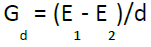
where d is the horizontal length used for the calculation of gradient (m), and E1 and E2 are elevations of upstream and downstream points [5].
Gd values for various d (160-9920) were calculated along each river. The results indicate that the gradients can be grouped into two major types: local and trend gradients. The local gradient with d<1200 shows a large fluctuation, reflecting local riverbed form. Such fluctuations decrease as d increases, and curves showing the trend gradient with d>1200 are much smoother. Example of stream gradients for various values of d (Karun River in central study area, subbasin 327) is shown in the Figure 5. Some statistical values of stream gradients (d=160-1120) for each river were calculated. The uppermost and lowermost 560-m reaches were excluded from the calculation because Gd for d=1120 could not be obtained. As the fluctuation of Gd decreases with increasing d, the standard deviation, maximum and range of Gd also decrease and the minimum Gd increase (Figures 6 and 7) (Tables 1-3). Unlike the local gradients, the trend gradients and the changing rates tend to increase with increasing d, which is particularly apparent when d exceeds ca. 6000. The standard deviation and range of Gd also increase with increasing d if d exceeds 6000. These facts seem to reflect the overall concavity of stream profiles. Because rivers generally take concave longitudinal profiles, Gd based on large d tends to be larger than that based on small d in the middle to lower reaches. Although the inverse is true for some upper reaches, the lengths are generally short. On the other hand, the standard deviation and range of Gd for d less than ca. 3000 decrease as d increases in the case of the local gradients. Therefore, Gd for d=ca. 3000-6000 can be regarded as the trend gradient suitable to this study. Because locally steep river segments have trend gradients less than the local gradients, we examined the rate of gradient change with increasing d as an indicator of relative steepness (Rd) of local river segments. As shown in Figure 8, some locations along a river show rapid decrease in Gd with increasing d when d is shorter than several thousand kilometers, and such locations seem to correspond to knickzones. Standard deviation of Gd for d=320-3040 except for the uppermost and lowermost 1520 m reaches was computed for each river, and the average was shown in Figure 8. For ca. d<1500, the standard deviation of Gd decreases as d increases, whereas for ca. d>1500, it increases with increasing d. The value of d at which the standard deviation is minimized was examined for each river; the average was 1805 m. This result is slightly different from the trend shown in Figure 6B, because of the inclusion of some uppermost and lowermost river segments (the uppermost and lowermost 1520 m reaches). The range of d from 320 to 1760 (the range of decreasing standard deviation with d) is, thus, regarded as the transition of the local to trend gradient (Figure 9).

Figure 5: Example of stream gradients for various values of d (Karun River in central study area, subbasin 327.

Figure 6: Mean (black circle) and standard deviation (vertical gray line) of statistical values of stream gradients (d=160-1120) for each river.

Figure 7: Statistical parameters and the changing rates of stream gradients (d=1280-9920 m).
| Mean Gd (m/m) | Minimum Gd (m/m) | Maximum Gd (m/m) | Standard deviation of Gd (m/m) | |
|---|---|---|---|---|
| d=160 | 0,00186 | -5,40125 | 0,49706 | 0,10005 |
| d=240 | 0,00184 | -3,45083 | 0,33146 | 0,07987 |
| d=320 | 0,00182 | -2,58750 | 0,26250 | 0,06856 |
| d=400 | 0,00181 | -2,05250 | 0,21885 | 0,06183 |
| d=480 | 0,00180 | -1,69167 | 0,18242 | 0,05620 |
| d=560 | 0,00179 | -1,44286 | 0,16071 | 0,05109 |
| d=640 | 0,00178 | -1,25625 | 0,14616 | 0,04775 |
| d=720 | 0,00177 | -1,11597 | 0,12994 | 0,04494 |
| d=800 | 0,00176 | -1,00375 | 0,11698 | 0,04254 |
| d=880 | 0,00176 | -0,91227 | 0,10636 | 0,04050 |
| d=960 | 0,00175 | -0,83594 | 0,09752 | 0,03886 |
| d=1040 | 0,00175 | -0,76971 | 0,09004 | 0,03728 |
| d=1120 | 0,00175 | -0,71429 | 0,08363 | 0,03592 |
Table 1: Statistical parameters and the changing rates of stream gradients (d=160-1120).
| Average Gd (*10-5 m/m) | Standard deviation of Gd (10-4 m/m) | |
|---|---|---|
| d=1280 | 167 | 2 |
| d=2240 | 167 | 2 |
| d=3200 | 167 | 2 |
| d=4160 | 167 | 2 |
| d=5120 | 168 | 2 |
| d=6080 | 169 | 3 |
| d=7040 | 170 | 4 |
| d=8000 | 171 | 5 |
| d=8960 | 172 | 7 |
| d=9920 | 174 | 11 |
Table 2: Statistical parameters and the changing rates of stream gradients (d=1280-9920 m).
| Change of average Gd (10-6 m/m2) | Change of standard deviation Gd (*10-5 m/m2) | |
|---|---|---|
| 1280-2240 | 0 | 2 |
| 2240-3200 | 2 | 2 |
| 3200-4160 | 6 | 2 |
| 4160-5120 | 8 | 3 |
| 5120-6080 | 8 | 5 |
| 6080-7040 | 10 | 6 |
| 7040-8000 | 10 | 10 |
| 8000-8960 | 20 | 21 |
| 8960-9920 | 20 | 46 |
Table 3: Statistical parameters and the changing rates of stream gradients for different values of d.

Figure 8: Gradient change with increasing d at a measurement point along Karun River.

Figure 9: Changes of standard deviation of stream gradients with d for d ≤ 3040.
Rd (m-1) for each location was measured by fitting a linear regression line to the relationship between d and Gd. An example of Rd distribution along a river is shown in Figure 10. The curve of Rd along the river shows fluctuations, in which relatively steep segments correspond to large values of Rd. The standard deviation of Rd for each river was examined, and its average for all the rivers was 1.42 × 10⁻⁵. River segments with Rd larger than this value were identified as knickzones (Figure 10), whereas those with height less than 10 m were excluded because the DEMs used in this study were constructed from topographic maps with 10-m contours. Relationship between fluvial knickpoint distribution and lithology in the study area was examined (Figure 11). Effects of rock properties on the frequency and form of knickzones are observed, but they seem to play only a subordinate role [5].

Figure 10: Longitudinal profile, relative steepness (Rd) and identified knickzones for Karun River. Gray dotted line shows a threshold value of Rd (1.42 × 10⁻⁵). Segments less than 10-m in height are not included in knickzones.

Figure 11: Relationship between fluvial knickpoint and lithology along river 201.
Fault movement potential
Study of quantitative seismotectonic parameters in a seismogenic area play an important role in the analysis of tectonic characteristics and earthquake potential in that area. Interrelationship between the tectonic stress field and crustal movement potential of any given area can be drawn by examining the principal stress orientations and the fault geometrical characteristics in that area, based on the Navier-Coulomb shear failure criterion [6]. In this paper the source parameters of 49 earthquakes with mb ≥ 4.0, from 1977 to 2010 [7], combined with information obtained from the fault maps have been analyzed to investigate the interrelationship between the Current Tectonic Regime (CTR) and the movement potential of the major faults in Khuzestan province. The overall orientation of the greatest principal stress was horizontal with an azimuth of NE-SW (Figure 12). Finally, the relationship between fluvial knickpoint distribution, active faults and maximum value of FMP in the study area was investigated (Figure 13) (Table 4) [8].

Figure 12: Maximum principal stress direction (σ1) in this study and previous study (Wyss, 1995).

Figure 13: Relationship between fluvial knickpoint distribution, active faults and maximum value of FMP in the study area.
| No | Zone | FD.DD | N.F | σ1 | µ | φ | θ0 | θf | (FMP)max | (FMP)avg |
|---|---|---|---|---|---|---|---|---|---|---|
| 1 | (32 45-33)(48- 48 15) | 90/268 | 0/88 | 06/035 | 0,3 | 16,7 | 53,35 | 56,73 | 0,99 | 0,84 |
| 2 | (32 45 33)(48 15-48 30) | 90/354 | 0/174 | 19/207 | 0,3 | 16,7 | 53,35 | 37,54 | 0,61 | 0,4 |
| 3 | (32 45-33)(48 30-48 45) | 90/354 | 0/174 | 19/207 | 0,3 | 16,7 | 53,35 | 37,54 | 0,69 | 0,55 |
| 4 | (32 45-33)(48 45-49) | 37/349 | 53/169 | 19/207 | 0,3 | 16,7 | 53,35 | 44,89 | 0,82 | 0,53 |
| 5 | (32 45-33)(49-49 15) | 53/220 | 37/40 | 06/104 | 0,3 | 16,7 | 53,35 | 65,73 | 0,92 | 0,72 |
| 6 | (32 45-33)(49 15-49 30) | 37/55 | 53/235 | 19/207 | 0,3 | 16,7 | 53,35 | 40,32 | 0,73 | 0,48 |
| 7 | (32 30-32 45)(47 45-48) | 90/11 | 0/191 | 2/224 | 0,3 | 16,7 | 53,35 | 33,05 | 0,96 | 0,78 |
| 8 | (32 30-32 45)(48-48 15) | 90/354 | 0/174 | 03/198 | 0,3 | 16,7 | 53,35 | 29,92 | 0,95 | 0,67 |
| 9 | (32 30-32 45)(48 15-48 30) | 53/67 | 37/247 | 13/193 | 0,3 | 16,7 | 53,35 | 56,35 | 0,97 | 0,7 |
| 10 | (32 30-32 45)(48 30-48 45) | 37/346 | 53/166 | 13/202 | 0,3 | 16,7 | 53,35 | 47,83 | 1 | 0,7 |
| 11 | (32 30-32 45)(48 45-49) | 53/93 | 37/273 | 16/201 | 0,3 | 16,7 | 53,35 | 66,23 | 0,74 | 0,58 |
| 12 | (32 30-32 45)(49-49 15) | 37/215 | 53/35 | 20/48 | 0,3 | 16,7 | 53,35 | 34,49 | 0,95 | 0,61 |
| 13 | (32 30-32 45)(49 15- 49 30) | 37/41 | 53/221 | 19/207 | 0,3 | 16,7 | 53,35 | 35,69 | 0,98 | 0,55 |
| 14 | (32 30-32 45)(49 30-49 45) | 37/55 | 53/235 | 19/207 | 0,3 | 16,7 | 53,35 | 40,32 | 0,93 | 0,64 |
| 15 | (32 15-32 30) (47 45-48) | |||||||||
| 16 | (32 15-32 30)(48-48 15) | 90/73 | 0/253 | 19/207 | 0,3 | 16,7 | 53,35 | 48,94 | 0,88 | 0,88 |
| 17 | (32 15-32 30)(48 15-48 30) | 37/27 | 53/207 | 19/207 | 0,3 | 16,7 | 53,35 | 34 | 0,47 | 0,47 |
| 18 | (32 15-32 30)(48 30-48 45) | |||||||||
| 19 | (32 15-32 30)(48 45-49) | 53/93 | 37/273 | 19/207 | 0,3 | 16,7 | 53,35 | 59,8 | 0,95 | 0,58 |
| 20 | (32 15-32 30)(49-49 15) | 37/34 | 53/214 | 19/207 | 0,3 | 16,7 | 53,35 | 34,43 | 0,97 | 0,64 |
| 21 | (32 15-32 30)(49 15-49 30) | 90/359 | 0/179 | 43/220 | 0,3 | 16,7 | 53,35 | 56,5 | 0,99 | 0,54 |
| 22 | (32 15-32 30)(49 30-49 45) | 37/47 | 53/227 | 19/207 | 0,3 | 16,7 | 53,35 | 37,37 | 1 | 0,57 |
| 23 | (32 15-32 30)(49 45-50) | 37/58 | 53/238 | 19/207 | 0,3 | 16,7 | 53,35 | 41,6 | 0,97 | 0,61 |
| 24 | (32-32 15)(47 30-47 45) | |||||||||
| 25 | (32-32 15)(47 45-48) | 37/48 | 53/228 | 19/207 | 0,3 | 16,7 | 53,35 | 37,7 | 0,98 | 0,55 |
| 26 | (32-32 15)(48-48 15) | 37/52 | 53/232 | 19/207 | 0,3 | 16,7 | 53,35 | 39,13 | 0,89 | 0,52 |
| 27 | (32-32 15)(48 15-48 30) | 53/108 | 37/288 | 19/207 | 0,3 | 16,7 | 53,35 | 71,7 | 0,93 | 0,59 |
| 28 | (32-32 15)(48 30-48 45) | 37/32 | 53/212 | 19/207 | 0,3 | 16,7 | 53,35 | 34,22 | 0,98 | 0,72 |
| 29 | (32-32 15)(48 45-49) | 90/93 | 0/273 | 12/049 | 0,3 | 16,7 | 53,35 | 67,38 | 0,97 | 0,71 |
| 30 | (32-32 15)(49-49 15) | 90/69 | 0/249 | 26/39 | 0,3 | 16,7 | 53,35 | 36,75 | 0,98 | 0,51 |
| 31 | (32-32 15)(49 15-49 30) | 37/29 | 53/209 | 19/207 | 0,3 | 16,7 | 53,35 | 34,04 | 1 | 0,57 |
| 32 | (32-32 15)(49 30-49 45) | 90/194 | 0/14 | 11/052 | 0,3 | 16,7 | 53,35 | 39,33 | 0,99 | 0,68 |
| 33 | (32-32 15)(49 45-50) | 90/82 | 0/242 | 19/207 | 0,3 | 16,7 | 53,35 | 39,24 | 0,98 | 0,55 |
| 34 | (32-32 15)(50-50 15) | 90/58 | 0/238 | 19/207 | 0,3 | 16,7 | 53,35 | 35,86 | 0,95 | 0,7 |
| 35 | (31 45-32)(47 30-47 45) | |||||||||
| 36 | (31 45-32)(47 45-48) | 37/48 | 53/228 | 19/207 | 0,3 | 16,7 | 53,35 | 37,7 | 0,57 | 0,57 |
| 37 | (31 45-32)(48-48 15) | 37/48 | 53/228 | 19/207 | 0,3 | 16,7 | 53,35 | 37,7 | 0,9 | 0,57 |
| 38 | (31 45-32)(48 15-48 30) | 53/90 | 37/180 | 19/207 | 0,3 | 16,7 | 53,35 | 29,69 | 0,9 | 0,57 |
| 39 | (31 45-32)(48 30-48 45) | 37/209 | 53/29 | 02/051 | 0,3 | 16,7 | 53,35 | 54,16 | 0,98 | 0,71 |
| 40 | (31 45-32)(48 45-49) | 37/55 | 53/235 | 06/049 | 0,3 | 16,7 | 53,35 | 84,34 | 0,99 | 0,68 |
| 41 | (31 45-32)(49-49 15) | 37/45 | 53/225 | 10/213 | 0,3 | 16,7 | 53,35 | 44,08 | 0,97 | 0,67 |
| 42 | (31 45-32)(49 15-49 30) | 53/159 | 37/339 | 02/047 | 0,3 | 16,7 | 53,35 | 68,1 | 1 | 0,84 |
| 43 | (31 45-32)(49 30-49 45) | 37/217 | 53/37 | 11/047 | 0,3 | 16,7 | 53,35 | 41,81 | 0,95 | 0,54 |
| 44 | (31 45-32)(49 45-50) | 90/66 | 0/246 | 19/207 | 0,3 | 16,7 | 53,35 | 42,71 | 0,98 | 0,68 |
| 45 | (31 45-32)(50-50 15) | 90/58 | 0/238 | 09/206 | 0,3 | 16,7 | 53,35 | 33,11 | 0,95 | 0,59 |
| 46 | (31 45-32)(50 15-50 30) | 37/57 | 53/237 | 19/207 | 0,3 | 16,7 | 53,35 | 41,17 | 0,95 | 0,62 |
| 47 | (31 30-31 45)(47 30-47 45) | |||||||||
| 48 | (31 30-31 45)(47 45-48) | |||||||||
| 49 | (31 30-31 45)(48-48 15) | 37/33 | 53/213 | 19/207 | 0,3 | 16,7 | 53,35 | 34,32 | 0,98 | 0,54 |
| 50 | (31 30-31 45)(48 15-48 30) | 90/62 | 0/242 | 19/207 | 0,3 | 16,7 | 53,35 | 39,24 | 0,97 | 0,65 |
| 51 | (31 30-31 45)(48 30-48 45) | 90/329 | 0/149 | 19/207 | 0,3 | 16,7 | 53,35 | 59,93 | 0,98 | 0,67 |
| 52 | (31 30-31 45)(48 45-49) | 90/348 | 0/168 | 19/207 | 0,3 | 16,7 | 53,35 | 42,71 | 0,71 | 0,71 |
| 53 | (31 30-31 45)(49-49 15) | 90/348 | 0/168 | 19/207 | 0,3 | 16,7 | 53,35 | 42,71 | 0,71 | 0,58 |
| 54 | (31 30-31 45)(49 15-49 30) | 53/168 | 37/348 | 07/052 | 0,3 | 16,7 | 53,35 | 76,85 | 0,95 | 0,73 |
| 55 | (31 30-31 45)(49 30-49 45) | 90/353 | 0/173 | 6/222 | 0,3 | 16,7 | 53,35 | 49,27 | 0,91 | 0,79 |
| 56 | (31 30-31 45)(49 45-50) | 90/358 | 0/178 | 69/221 | 0,3 | 16,7 | 53,35 | 74,81 | 1 | 0,6 |
| 57 | (31 30-31 45)(50-50 15) | 37/2 | 53/182 | 19/207 | 0,3 | 16,7 | 53,35 | 39,13 | 0,98 | 0,57 |
| 58 | (31 30-31 45)(50 15-50 30) | 53/100 | 37/280 | 14/181 | 0,3 | 16,7 | 53,35 | 88,6 | 0,97 | 0,63 |
| 59 | (31 15-31 30)(47 30-47 45) | |||||||||
| 60 | (31 15-31 30)(47 45-48) | |||||||||
| 61 | (31 15-3130)(48-48 15) | 37/33 | 53/213 | 19/207 | 0,3 | 16,7 | 53,35 | 34,32 | 0,9 | 0,69 |
| 62 | (31 15-31 30)(48 15-48 30) | 37/33 | 53/213 | 19/207 | 0,3 | 16,7 | 53,35 | 34,32 | 0,95 | 0,57 |
| 63 | (31 15-31 30)(48 30-48 45) | 37/36 | 53/216 | 19/207 | 0,3 | 16,7 | 53,35 | 34,71 | 0,56 | 0,52 |
| 64 | (31 15-31 30)(48 45-49) | |||||||||
| 65 | (31 15-31 30)(49-49 15) | 90/66 | 0/246 | 19/207 | 0,3 | 16,7 | 53,35 | 42,71 | 0,71 | 0,71 |
| 66 | (31 15-31 30)(49 15-49 30) | 37/8 | 53/188 | 19/207 | 0,3 | 16,7 | 53,35 | 37,06 | 0,73 | 0,62 |
| 67 | (31 15-31 30)(49 30-49 45) | 37/8 | 53/188 | 19/207 | 0,3 | 16,7 | 53,35 | 37,06 | 0,64 | 0,47 |
| 68 | (31 15-31 30)(49 45-50) | 37/42 | 53/222 | 19/207 | 0,3 | 16,7 | 53,35 | 35,94 | 0,81 | 0,58 |
| 69 | (31 15-31 30)(50-50 15) | 53/90 | 37/270 | 19/207 | 0,3 | 16,7 | 53,35 | 57,4 | 0,89 | 0,6 |
| 70 | (31 15-31 30)(50 15-50 30) | 37/57 | 53/237 | 19/207 | 0,3 | 16,7 | 53,35 | 41,17 | 0,95 | 0,6 |
| 71 | (31-31 15)(47 30-47 45) | |||||||||
| 72 | (31-31 15)(47 45-48) | |||||||||
| 73 | (31-31 15)(48-48 15) | |||||||||
| 74 | (31-31 15)(48 15-48 30) | |||||||||
| 75 | (31-31 15)(48 30-48 45) | 37/36 | 53/216 | 19/207 | 0,3 | 16,7 | 53,35 | 34,71 | 0,49 | 0,49 |
| 76 | (31-31 15)(48 45-49) | 37/36 | 53/216 | 19/207 | 0,3 | 16,7 | 53,35 | 34,71 | 0,49 | 0,49 |
| 77 | (31-31 15)(49-49 15) | |||||||||
| 78 | (31-31 15)(49 15-49 30) | 90/58 | 0/238 | 19/207 | 0,3 | 16,7 | 53,35 | 35,86 | 0,78 | 0,55 |
| 79 | (31-31 15)(49 30-49 45) | 53/122 | 37/302 | 19/207 | 0,3 | 16,7 | 53,35 | 82,52 | 0,6 | 0,41 |
| 80 | (31-31 15)(49 45-50) | 90/100 | 0/280 | 7/243 | 0,3 | 16,7 | 53,35 | 37,56 | 0,97 | 0,69 |
| 81 | (31-31 15)(50-50 15) | |||||||||
| 82 | (30 45-31)(48-48 15) | |||||||||
| 83 | (30 45-31)(48 15-48 30) | |||||||||
| 84 | (30 45-31)(48 30-48 45) | |||||||||
| 85 | (30 45-31)(48 45-49) | 90/69 | 0/249 | 19/207 | 0,3 | 16,7 | 53,35 | 45,36 | 0,78 | 0,78 |
| 86 | (30 45-31)(49-49 15) | 90/69 | 0/249 | 19/207 | 0,3 | 16,7 | 53,35 | 45,36 | 0,78 | 0,78 |
| 87 | (30 45-31)(49 15-49 30) | 90/72 | 0/252 | 19/207 | 0,3 | 16,7 | 53,35 | 48,04 | 0,86 | 0,86 |
| 88 | (30 45-31)(49 30-49 45) | 37/56 | 53/236 | 19/207 | 0,3 | 16,7 | 53,35 | 40,74 | 0,86 | 0,54 |
| 89 | (30 45-31)(49 45-50) | 90/174 | 0/354 | 14/40 | 0,3 | 16,7 | 53,35 | 47,62 | 0,84 | 0,65 |
| 90 | (30 45-31)(50-50 15) | 53/100 | 37/280 | 13/206 | 0,3 | 16,7 | 53,35 | 69,52 | 0,75 | 0,64 |
| 91 | (30 45-31)(50 15-50 30) | 53/323 | 37/143 | 19/207 | 0,3 | 16,7 | 53,35 | 58,2 | 0,87 | 0,87 |
| 92 | (30 30-30 45)(48-48 15) | 37/6 | 53/186 | 19/207 | 0,3 | 16,7 | 53,35 | 37,7 | 0,57 | 0,57 |
| 93 | (30 30-30 45)(48 15-48 30) | 37/6 | 53/186 | 19/207 | 0,3 | 16,7 | 53,35 | 37,7 | 0,63 | 0,4 |
| 94 | (30 30-30 45)(48 30-48 45) | |||||||||
| 95 | (30 30-30 45)(48 45-49) | 53/327 | 37/147 | 19/207 | 0,3 | 16,7 | 53,35 | 55,01 | 0,95 | 0,95 |
| 96 | (30 30-30 45)(49-49 15) | 90/69 | 0/249 | 19/207 | 0,3 | 16,7 | 53,35 | 45,36 | 0,78 | 0,78 |
| 97 | (30 30-30 45)(49 15-49 30) | 90/72 | 0/252 | 19/207 | 0,3 | 16,7 | 53,35 | 48,04 | 0,86 | 0,86 |
| 98 | (30 30-30 45)(49 30-49 45) | 90/72 | 0/252 | 19/207 | 0,3 | 16,7 | 53,35 | 48,04 | 0,93 | 0,83 |
| 99 | (30 30-30 45)(49 45-50) | 53/333 | 37/153 | 19/207 | 0,3 | 16,7 | 53,35 | 50,22 | 0,91 | 0,69 |
| 100 | (30 30-30 45)(50-50 15) | 37/229 | 53/49 | 04/048 | 0,3 | 16,7 | 53,35 | 49,01 | 0,88 | 0,53 |
| 101 | (30 30-30 45)(50 15-50 30) | 37/38 | 53/218 | 19/207 | 0,3 | 16,7 | 53,35 | 35,06 | 0,76 | 0,47 |
| 102 | (30 15-30 30)(48-48 15) | |||||||||
| 103 | (30 15-30 30)(48 15-48 30) | 53/102 | 37/282 | 19/207 | 0,3 | 16,7 | 53,35 | 66,96 | 0,63 | 0,31 |
| 104 | (30 15-30 30)(48 30-48 45) | 53/327 | 37/147 | 19/207 | 0,3 | 16,7 | 53,35 | 55,01 | 0,95 | 0,95 |
| 105 | (30 15-30 30)(48 45-49) | 53/327 | 37/147 | 19/207 | 0,3 | 16,7 | 53,35 | 55,01 | 0,95 | 0,95 |
| 106 | (30 15-30 30)(49-49 15) | 53/327 | 37/147 | 19/207 | 0,3 | 16,7 | 53,35 | 55,01 | 0,95 | 0,91 |
| 107 | (30 15-30 30)(49 15-49 30) | 53/327 | 37/147 | 19/207 | 0,3 | 16,7 | 53,35 | 55,01 | 0,95 | 0,91 |
| 108 | (30 15-30 30)(49 30-49 45) | 53/327 | 37/147 | 19/207 | 0,3 | 16,7 | 53,35 | 55,01 | 0,95 | 0,91 |
| 109 | (30 15-30 30)(49 45-50) | |||||||||
| 110 | (30 15-30 30)(50-50 15) | 53/120 | 37/300 | 19/207 | 0,3 | 16,7 | 53,35 | 81 | 0,9 | 0,6 |
| 111 | (30 15-30 30)(50 15-50 30) | 53/300 | 37/120 | 04/044 | 0,3 | 16,7 | 53,35 | 76,43 | 0,89 | 0,56 |
| 112 | (30-30 15)(48 15-48 30) | 53/102 | 37/282 | 19/207 | 0,3 | 16,7 | 53,35 | 66,96 | 0,63 | 0,31 |
| 113 | (30-30 15)(48 30-48 45) | |||||||||
| 114 | (30-30 15)(48 45-49) | |||||||||
| 115 | (30-30 15)(49-49 15) | |||||||||
| 116 | (30-30 15)(49 15-49 30) | 90/72 | 0/252 | 19/207 | 0,3 | 16,7 | 53,35 | 48,04 | 0,86 | 0,86 |
| 117 | (30-30 15)(49 30-49 45) | 90/75 | 0/255 | 19/207 | 0,3 | 16,7 | 53,35 | 50,75 | 0,93 | 0,93 |
| 118 | (30-30 15)(49 45-50) | |||||||||
| 119 | (30-30 15)(50-50 15) | 37/38 | 53/218 | 19/207 | 0,3 | 16,7 | 53,35 | 35,06 | 0,93 | 0,76 |
| 120 | (30-30 15)(50 15-50 30) | 37/4 | 53/184 | 19/207 | 0,3 | 16,7 | 53,35 | 58,41 | 0,91 | 0,89 |
Table 4: Results of maximum stress direction, fault movement potential in each zone.
Conclusion
Investigations on major mountain rivers revealed that knickzones are generally abundant in the study area. Knickzones with large relative steepness near the outlets of large watersheds are related to the tectonic activity and most of them are actually close to the known locations of active faults. Knickzones occur along upstream steep reaches can be related to active hydraulic and erosional conditions regardless of geological or tectonic conditions. Effects of rock properties on the frequency and form of knickzones are observed, but they seem to play only a subordinate role. This study concludes that tectonics and geology are more important than topographic and hydraulic conditions in knickzone existence. The Fault Movement Potential (FMP), one of the most important parameters related to seismicity assessment, evaluates the seismic hazard of fault systems, based on evaluation of fault activity by considering the mechanical relationships between fault geometry and regional tectonic stress field. FMP values are more consistent with the patterns of faults and present-day earthquake activity in the area. There also seems to be a good relationship between fluvial knickpoint distribution, seismotectonic zoning based on FMP and seismotectonic source of knickpoints.
Acknowledgement
This work was supported by the Behbahan branch of Islamic Azad University. We would like to thank this department.
References
- Sun C, Wan T, Xie X, Shen X, Liang K (2016) Knickpoint series of gullies along the Piedmont and its relation with fault activity since late Pleistocene. Geomorphol 268: 266-274.
- Grimaud JL, Paola C, and Voller V (2016) Experimental migration of knickpoints: inuence of style of base-level fall and bed lithology. Earth Surface Dyn 4: 11-23.
- Schmidt J, Zeitler P, Pazzaglia F, Tremblay M, Shuster D, et al. (2015) Knickpoint evolution on the Yarlung river: Evidence for late Cenozoic uplift of the southeastern Tibetan plateau margin. Earth and Planet Sci Letters 430: 448-457.
- Pavano F, Pazzaglia F, Catalano S (2016) Knickpoints as geomorphic markers of active tectonics: A case study from northeastern Sicily (south Italy). Geolo Society of America.
- Hayakawa YS, Oguchi T (2006) DEM-based identification of fluvial knickzones and its application to Japanese mountain rivers. Geomorphol 78: 90-106.
- Lee CF, Hou JJ, Ye H (1997) The movement potential of the major faults in Hong Kong area. Episod V 20: 33-52.
- Reshes Z (1978) Determination of the tectonic stress tensor from slip along faults that obey Coulomb yield condition. Tectonics 6: 849-861.
- Stocklin J (1968a) Structural history and tectonics of Iran: a review: AAPG Bulletin 52: 1229-1258.
Relevant Topics
- Algal Blooms
- Blue Carbon Sequestration
- Brackish Water
- Catfish
- Coral Bleaching
- Coral Reefs
- Deep Sea Fish
- Deep Sea Mining
- Ichthyoplankton
- Mangrove Ecosystem
- Marine Engineering
- Marine Fisheries
- Marine Mammal Research
- Marine Microbiome Analysis
- Marine Pollution
- Marine Reptiles
- Marine Science
- Ocean Currents
- Photoendosymbiosis
- Reef Biology
- Sea Food
- Sea Grass
- Sea Transportation
- Seaweed
Recommended Journals
Article Tools
Article Usage
- Total views: 4474
- [From(publication date):
February-2017 - Jul 16, 2025] - Breakdown by view type
- HTML page views : 3508
- PDF downloads : 966