Research Article Open Access
Effect of Initial Pressure, Surface, Outlet Velocity, and Density of Adsorbed Gas on Transport and Production in Shale Gas Reservoirs
Balumi WB1* and Aminu MD21Department of Geology, Federal University, Birnin Kebbi, Nigeria
2Department of Geology, Modibbo Adama University of Technology, Yola, Nigeria
- *Corresponding Author:
- Balumi WB
Department of Geology
Federal University
Birnin Kebbi, Nigeria
Tel: +234 700 000 000
E-mail: wakilbalumi@hotmail.com
Received date: July 19, 2017; Accepted date: August 08, 2017; Published date: August 14, 2017
Citation: Balumi WB, Aminu MD (2017) Effect of Initial Pressure, Surface, Outlet Velocity, and Density of Adsorbed Gas on Transport and Production in Shale Gas Reservoirs. Oil Gas Res 3: 144. doi: 10.4172/2472-0518.1000144
Copyright: © 2017 Balumi WB, et al. This is an open-access article distributed under the terms of the Creative Commons Attribution License, which permits unrestricted use, distribution, and reproduction in any medium, provided the original author and source are credited.
Visit for more related articles at Oil & Gas Research
Abstract
The recent technological advancements in horizontal drilling and hydraulic fracturing have led to a boom in gas production from unconventional shale gas reservoirs. However, knowledge and technologies required to successfully develop unconventional reservoirs are far beyond what is available in the industry at present. Shale gas reservoirs are extremely heterogeneous with ultra-low permeability and nano-pores. The flow of gas in this reservoir is non-linear, multi-faceted including adsorption/desorption, flow at high and low rates, solid-fluid interactions, etc., which makes it a significant challenge to quantify such flow. A pore-scale flow model was developed using a combination of CFD and COMSOL multi-physics 4.2 based on Darcy and Navier-Stokes equations to describe transport of adsorbed gas and free gas in pore spaces respectively. Parameters such as surface pressure, adsorbed gas density and initial reservoir pressure were used to study shale gas transport. The presence of adsorbed gas within the shale gas reservoir will decrease porosity while increasing total production and gas storage capacity due to the high affinity of surfaces of organic matter to methane found within the shale gas reservoirs and hence high gas-in-place estimates. Moreover, because production from the adsorbed gas phase is dependent on pressure, four different values of initial reservoir pressures were used to analyze the effect of reservoir pressure on flow velocity. It was observed that the higher the initial reservoir pressure, the greater the velocity of the flow and consequently higher production rates.
Keywords
Unconventional; Shale gas; Reservoirs; Permeability; Nanopores; Darcy equation; Navier-stokes equation
Abbreviations
CAD: Computer Aided Design; CFD: Computational Fluid Dynamics; DXF: Drawing Exchange Format; FIB: Focused ion beam; GIP: Gas Initially in Place; SEM: Scanning Electron Microscope
Introduction
To achieve commercial production in unconventional reservoirs, stimulation of the reservoir is required. These types of reservoirs require fracture stimulation to release the vast amount of oil and gas stored in very low-permeability formations such as shale. Different processes combine to control gas storage and flow in shale gas reservoirs. Gas storage is achieved as compressed gas in pore spaces, as gas adsorbed on to the walls of pores, organic matter, clays etc., and in solid organic materials such as kerogen and clays where it exists as a soluble gas. The flow of gas in shale is achieved through a network of pores with different diameters ranging from nano-meters to micrometers [1,2]. These nanopores are important because of the following reasons:
(1) The surface area exposed is larger in nanopores than in micropores for the same pore volume. Since surface area is proportional to 4/d, where d=pore diameter, this large surface exposed leads to large volume of gas desorption from surfaces of the kerogen.
Gas flow in shale is through nanopores, which does not follow Darcy flow.
(2) This study was carried out to account for the contribution of adsorption phenomena in shale to production and gas initially in place (GIP) at pore scale. It is also aimed at improving our understanding of pore scale transport in shale gas reservoirs in general.
Materials and Methods
Sample preparation
The methodology for this study is divided into two: firstly, the creation of a pore-scale finite element mesh of shale rock from scanning electron microscope (SEM) images and secondly, the numerical simulation of shale gas transport at pore-scale level based on published reservoir data obtained from production and well completion of shale formation.
SEM imaging and grey scale imaging
Scanning electron microscope is an electronic microscope that uses a concentration of electrons to generate different signals at the surface of the shale sample under investigation. These signals reveal salient information about the sample such as texture, structure and grain orientation within the sample. Greyscale imaging which consists of variety of grey shades devoid of any obvious color are the most preferred format for image processing. Sometimes white shades may appear as the brightest shades possible indicating the total presence of light within the visible wavelengths. Black shades where present similarly indicate the darkest shade possible and the complete absence of light in such images. Brightness levels of equal measures including three major colors such as green, blue and red are used to represent intermediate shades of grey for reflected lights. Measurement techniques such as focused ion beam (FIB) and scanning electron microscopy are capable of direct measurement and visualization of shale matrix at nano-scale on high quality flat surfaces, thereby providing a new insight on the nano-scale structures available in shale matrix. Figures 1 and 2 show SEM images, revealing area of interest and etched geometric patterns in silicon wafer.

Figure 1: SEM images showing areas of interest.

Figure 2: SEM image of etched geometric patterns in silicon wafer [2].
CFD Modeling Using SEM Technique
The initial phase in modeling the transport of shale gas in inorganic component of shale using computational fluid dynamics (CFD) modeling is the construction of pore-scale finite element mesh using FIB or SEM, reproduced using a computer-based drawing program. The generation of finite volume mesh model from FIB/SEM is preceded by importation of the images into COMSOL Multiphysics software prior to converting them into solids from computer aided design (CAD) format. The model is subsequently reworked and defined again to bring about the finite volume meshing. To avoid unnecessary errors during the modeling process, the geometric profile and the ultimate meshing of the model must be precisely defined. This is followed by the definition of flow fields and importation of files into COMSOL Multiphysics software to assist in bringing solutions to complex flow equations. Parameters and variables such as flow domain, fluid properties, output pressure, etc., are inputted to solve the flow relationships in the software. Using the fundamentals of fluid dynamics and by delineating boundary conditions, COMSOL Multiphysics software solves the numerical variables [3]. Figure 3 shows kerogen content (shown as dark areas) and inorganic constituents (represented in grey color) within the Barnett shale, using SEM imaging (Figure 4).

Figure 3: SEM image of the Barnett Shale [4].

Figure 4: Different levels of conversion of rock SEM image to pore scale finite element calculation mesh.
Definition of the model
The model covers an area of 6.4 × 10-4 m × 3.3 × 10-4 m (Figure 5). The flow of gas within the model is usually from the right-hand side to the left-hand side across the model geometry. Laminar flow is assumed in the pores and the gas does not go into the grains in the matrix. Fluid pressures at the inlet (Figure 6 and Table 1) and outlet (Figure 7, Tables 2 and 3) are known and defined. Symmetric gas flow is also assumed at the top and bottom boundaries. The main area of interest is rectangular with its topmost left corner set at (0,0) μm and lower most right coordinates set at (5.6, 2.3) × 10-4 Gravity has not being accounted for in this model due to its small-scale dimensions. The physical boundaries of the model can be mathematically represented by the equations used. The inlet and outlet pressures are known, to achieve a no-slip condition the velocities at grain boundaries are set as zero. The flow around the lower and upper boundaries is symmetric. Figure 8 depicts walls within the boundaries in the model, and Table 3 is a presentation of conditions at boundaries. Table 4 shows parameters for the model. The mathematical description for the detailed fluid mechanics in the interstitial pore space is based on the assumptions that we have steady state flow in isothermal conditions and the fluid is continuum, Newtonian, and incompressible (Figures 5 and 6).

Figure 5: A 6.4 × 10-4 m × 3.3 × 10-4 m geometry and boundary conditions.

Figure 6: Inlet boundary of the model.

Figure 7: Outlet boundaries of the model.

Figure 8: Walls within the boundaries in the model.
| Description | Value |
|---|---|
| Boundary condition | Pressure |
| Pressure | p0 |
| Suppress backflow | On |
| Flow direction | Normal flow |
| Use weak constraints | Off |
| Apply reaction terms on | All physics (symmetric) |
| Constraint method | Elemental |
Table 1: Inlet boundary settings used in the model.
| Description | Value |
|---|---|
| Boundary condition | Pressure |
| Pressure | 0 |
| Normal flow | Off |
| Suppress backflow | On |
| Use weak constraints | Off |
| Apply reaction terms on | All physics (symmetric) |
| Constraint method | Elemental |
Table 2: Outlet boundary settings used in the model.
| Type of Boundary | Condition of the Boundary | Value |
|---|---|---|
| Outlet Boundary | Pressure, P | p=0 |
| Inlet Boundary | Pressure, P | p=P0 |
| Sides of the Symmetry | Symmetric | Nil |
| Walls of the grain | - | Zero slip |
Table 3: Conditions at boundaries of the model. Note: where P0=change in pressure.
| Name | Expression | Value |
|---|---|---|
| rho | 0.67 (kg/m3) | 0.67000 kg/m³ |
| mu | 10.99E-6 (Pa*s) | 1.0990E-5 Pa·s |
| p0 | 2000 (kPa) | 2.0000E6 Pa |
Table 4: Model parameters.
Initial and boundary conditions
The pressure distribution of the shale gas pore system at a time t=0 defines the initial condition. This distribution of pressure is assumed to be the same all through the shale formation and is equivalent to the initial pressure of the reservoir. The concentration of the shale gas on the surface of pores and matrix within the system is assessed at the pore scale level. The pore system is specified using the boundary conditions along the pores within the system.
Governing Equations
Navier-stokes equation
By assuming a constant temperature and fluid density in the pores of the rock, Navier-Stokes and continuity equation can be used as follows [4,5].
ρ (∇u ⋅∇u) = ∇. − pIη∇u (∇u)T) = ∇⋅ u = 0 (1)
Where,
η: Dynamic viscosity (kg/(m·s)),
μ: Velocity (m/s),
ρ: Fluid density (kg/m3),
p: Pressure (Pa),
I: Identity matrix.
Darcy law with adsorption
The flow of gas and its transport processes in porous formations can be described mathematically from the principle of mass conservation of fluid/solute and Newton’s 2nd law of motion [6]. The general equation for conservation of mass or volume in porous media is as follows:(rate of mass inflow)-(rate of mass out flow)+(rate of mass production/ production)=(rate of mass accumulation) (Table 5). Desorption of shale gas from the surface of pores is followed by diffusion through the shale matrix until a fracture is met, after which the gas flow is based on Darcy law. This statement of mass conservation can be combined with a mathematical expression of relevant process to obtain a differential equation that will describe flow or transport in shale gas reservoirs. Per Darcy’s law for flow in a porous medium, the absolute permeability of the present model can be numerically calculated. The seepage or superficial velocity in horizontal direction can be obtained from the following expression [7].
 (2)
(2)
From Equation (11), K (absolute permeability) can be easily estimated. Darcy’s Law is valid for the slow flow (inertial effects can be neglected) of a Newtonian fluid through a porous medium with rigid solid matrix.
 (3)
(3)
Where,
V: Velocity of the fluid in the formation
K: Permeability of the rock
ρ: Fluid density
μ: Fluid viscosity
∇P: Pressure gradient
 : Rate of change in mass in control volume.
| Property | Value |
|---|---|
| Minimum element quality | 3.08E-04 |
| Average element quality | 0.7342 |
| Triangular elements | 13352 |
| Quadrilateral elements | 4634 |
| Edge elements | 2456 |
| Vertex elements | 2232 |
| Calibrate for | Fluid dynamics |
| Maximum element size | 1.6 |
| Minimum element size | 0.048 |
| Curvature factor | 0.25 |
| Maximum element growth rate | 1.08 |
| Predefined size | Extra fine |
| Custom element size | Custom |
Table 5: The table presents statistics of mesh used in the model, while other parameters used in the model which were selected based on published literature review on shale gas simulation [5,8] is tabulated in Table 6.
Conceptual flow models in shale can be single or two phase flow model based on the fluid content in the formation under study. Moreover, because we are mostly concerned with the transport of the gas in the reservoir, we can assume the system is immobile and has residual water saturation. This will simplify the formulation of the model into a single-phase flow. This single-phase flow can be further categorized into two based on the presence or absence of adsorption/ desorption as follows [8].
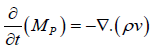 (4)
(4)
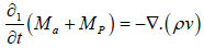 (5)
(5)
Where,
Ma: Amount of mass present in adsorbed state
Mp: Amount of gas present in the pores in the formation
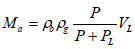
The mass of adsorbed gas in the formation can be expressed as follows:
 (6)
(6)
Where,
ρb: Bulk density of the rock
ρa: Gas density at standard condition
Va: Adsorbed gas volume based on Langmuir adsorption isotherm.
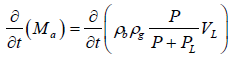
By simply replacing Va with VE and substituting  into
equation (6) we get:
into
equation (6) we get:
 (7)
(7)
 (8)
(8)
By taking away the constants
 (9)
(9)
 (10)
(10)
Hence
 (11)
(11)
Mass of gas in the reservoir pore volume can be expressed as a function of the porosity of the reservoir and the density of the fluid in the reservoir:
 (12)
(12)
Where,
 Reservoir porosity
Flow of free and adsorbed gas in a shale matrix can be described using the following expression:
 (13)
(13)
Where,
v: Darcy velocity
MT: Total mass of gas in the shale formation:
MT: Mads+Mfree (14)
Mads: Mass of adsorbed gas in the shale formation
Mass of free gas in the shale formation
Mfree: The masses of adsorbed gas and free gas are given by the following equations:
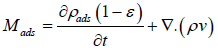 (15)
(15)
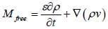 (16)
(16)
The total flow in the organic-inorganic matrix system in shale can be represented by:
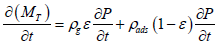 (17)
(17)
By rearranging and including the velocity term, we obtain the following:
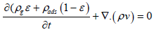 (18)
(18)
Assumptions of the model
The model developed for this study is based on the following key assumptions:
I. A single-phase flow is present in the model,
II. Temperature in the reservoir is constant throughout the reservoir always,
III. Permeability is assumed to be the same throughout the formation,
IV. The gas obeys ideal gas laws,
V. The formation is uniform and rectangular,
VI. The effect of heterogeneity and gravity on gas flow are neglected,
VII. Gas adsorption-desorption is based on Langmuir curve.
Implementation of the model
COMSOL Multi physics software has a fluid flow physics interface (based on Darcy’s law interface) which when selected along with the time dependent study type in a model can be used to solve the above flow equations used to describe the flow of gas in shale formations. Material properties such as density, permeability, porosity, etc., are inferred using the imported image in this model. The mesh setting was used to separate the model into several tiny triangular and rectangular shapes as shown below in Figure 9.

Figure 9: Mesh setting to separate model into several tiny triangular and rectangular shapes.
Results and Discussions
In this work, we investigated the effect of parameters such as initial reservoir pressure, surface velocity, outlet velocity and the contribution of free and adsorbed gas on gas transport and production in shale gas reservoirs. These parameters are added to the model created to investigate their effect on fluid flow and production in shale formation.
Single phase flow without adsorption
Initial reservoir pressure is the sole driving force in gas reservoirs and as such it is very essential to transport and production in gas reservoirs. Here the effect of initial reservoir pressure on gas transport is considered. Four different values of initial reservoir pressure - 500 KPa, 1000 KPa, 1500 KPa, and 20 KPa were considered as shown in Figure 10 at pore scale level. While varying the pressure during the investigations the other parameters shown in Table 6 are kept constant. Figure 10 shows the solution estimated using Navier-Stoke analysis for fluid velocity field in the pore spaces of a micro-porous shale formation. Higher velocity magnitudes which are indicated by the red and cyan shades of color are concentrated on the narrowest pores within the slide as the gas is moving from the inlet to the outlet as shown by the arrows, this decreases as the fluid moves towards the outlet due to the increase in cross sectional area available for flow. Around the midsection of the slides, a high velocity magnitude is recorded within a wider area which reveals that at relatively lower pressures when multiple channels commingle at a central point, high velocity magnitudes are obtained. The highest flow velocity is several times greater than the lowest flow velocity within the shale sample. This high velocity streamlines are believed to represent the favored path for gas flow in the model. When the initial reservoir pressure was increased 100%, the surface velocity was also doubled. This will consequently mean an increase in production of shale gas. Figure 11 gives the pressure contours across the sample slide at 2000 kPa. The figure clearly shows the reduction in pressure across the slide from the inlet to the outlet. The highest pressure occurs at the inlet while the lowest pressure occurs at the outlet in the sample shown below. Since gases always travel from high velocity area to low velocity areas, a high flow rate and production rate is expected from this model. Figure 12 shows a domain plot that explains the x-velocity at the four different pressures within the outlet. Because the flow is moving in the negative side of the x-axis, the velocities are assigned negative values. This buttresses the points raised above. Surface pressure plot of the model is shown in Figure 13. Maximum pressure occurs at the inlet as the gas travels because of pressure gradient and the pressure at the edge of the inlet is several folds greater than the pressure at the outlet within the boundaries of domain. This in addition to the results discussed above further shows the importance of initial reservoir pressure as the driving force within shale gas reservoirs.

Figure 10: Surface velocity fields with arrow plots computed using Navier- Stokes equation at four different initial reservoir pressures.

Figure 11: Pressure contour plot showing pressure distributions within the slide.

Figure 12: Domain plot showing velocities at the outlet boundaries using four different initial reservoir pressure values.

Figure 13: Surface pressure plots of the model at four different initial reservoir pressure values.
| Name | Expression | Value |
|---|---|---|
| V_std | 0.0224 (m3/mol) | 0.022400 m³/mol |
| M | 0.016 (kg/mol) | 0.016000 kg/mol |
| rho_s | 2560 (kg/m3) | 2560.0 kg/m³ |
| PL | 3.05e6 (1/Pa) | 3.0500E6 1/Pa |
| VL | 9.80E-4 (m3/kg) | 9.8000E-4 m³/kg |
| k | 1.0E-19 (m2) | 1.0000E-19 m² |
| epsilon | 0.5 | 0.5 |
| rho_g | 0.66 (kg/m3) | 0.66000 kg/m³ |
| mu | 0.0184 (cP) | 1.8400E-5 Pa·s |
Table 6: More parameters used in the model.
Single phase flow with adsorbed gas
The Langmuir isotherm describes the effect of pressure on adsorption in shale gas reservoirs based on a Langmuir volume and Langmuir pressure of 9.8000e-4 m³/kg and 3.0500e6 Pa respectively. Fluid viscosity at initial reservoir condition is 0.01804 cp. The effect of adsorption on pore size and transport in shale gas reservoirs was also considered. It is important to note that in this work we compared a situation where adsorption is considered and where it is ignored. Where adsorption was ignored, only free gas in the rock matrix was considered. Adsorption in shale gas reservoir could lead to the modification of the porosity and permeability of the reservoir rock as the reservoir is being depleted and its pressure gradient is reduced [9]. The pressure across the surface of the sample is less than 0.50E7 Pa as shown in Figure 14. The effect of adsorption on shale gas transport depends on pressure within the matrix of the rock. This low pressure means low adsorbed gas density and volume. Total gas production in a shale gas reservoir is the sum of adsorbed gas within surfaces in the rock and free gas found in the pores, and natural fractures. Moreover, any analysis of the producible gas within a shale gas reservoir must include desorption, and failure to do so will result in erroneous estimate. The density of the gas is usually affected by the interaction of the gas molecules with its environment and this depends on the nature of the surface of the matrix and its bulk material properties. The density of adsorbed gas is found to be much lesser than that of the free gas, but by not considering it during analysis and estimations of GIP, a very significant volume of gas production will be neglected. For example, in comparing the free gas and adsorbed gas density across the surface of the sample, free gas had a density of 3.3e-1 Kg/m3 while adsorbed gas had a density of -2.97e-7 Kg/m3, as such, based on this comparison we can see that adsorbed gas has a considerably lower density than the free gas but it is still significant for consideration in any analysis of gas production in shale gas reservoirs.

Figure 14: Surface gas pressure across the sample at pore-scale.
Summary of Findings
This study presents the result of numerical simulation of gas transport and the effect of adsorption on production in shale gas reservoirs. Initially, SEM image of the shale sample was converted to a grey image of the pore-scale finite element mesh. The CAD image formed was imported into COMSOL Multiphysics 4.2 and the organic components of the shale removed to form a pore scale model. The flow fields were defined to obtain accurate solutions to complex flow equations by delineating boundary conditions and using fundamentals of fluid dynamics in COMSOL Multiphysics software to solve for the numerical variables. Pore-scale modelling was carried out by describing the morphology of the porous medium and subsequently importing the SEM image as drawing exchange format (DXF) file into COMSOL Multiphysics software. The outlined software was then used to simulate the effect of initial reservoir pressures, surface pressures and adsorption on gas transport using the fluid flow module in the software. The transport of single phase gas in the pore space was described based on Navier-Stokes equation while fluid flow incorporating free and adsorbed gas was described based on Darcy law. The direction of gas flow in the model was set from the right-hand side to the left-hand side based on several assumptions that were meant to further validate and simplify the difficulties to be encountered. Parameters such as fluid pressure, inlet and outlet pressures were known and defined. At time t=0, the pressure distribution in the shale gas pore system was defined as the initial condition. This was assumed to be the same throughout the formation and it’s the same as the initial pressure of the reservoir. The effect of initial reservoir pressure, surface velocity, outlet velocity and density of adsorbed gas on gas transport and production was studied. The analysis of the results was divided into two based on single phase flow transport where the effect of adsorption was considered and where the effect of adsorption was ignored (in which only free gas in the rock matrix was considered). Furthermore, in analyzing single phase flow without adsorption four different values of initial reservoir pressures were used to gauge the effect of the parameter on shale gas transport and production. The results showed that a direct relationship exists between the initial reservoir pressure and velocity of the shale gas within the pores in the shale reservoir and hence the greater the initial reservoir pressure, the higher the velocity of the shale gas and consequently the greater the production. The effect of adsorption on single phase flow was considered based on surface pressure and density of the adsorbed gas and a comparison was made between the density of adsorbed gas and free gas. Hence, considering the effect of desorption in any analysis of shale gas reservoirs will lead to more accurate estimates of total gas production. The following conclusions were drawn from this study:
i. High velocity magnitudes are concentrated on the narrowest pore channels and at junctions where there is a commingling of channels within the shale formation. This high velocity channels are believed to be the preferred channel for shale gas transport.
ii. Initial reservoir pressure has a hugely significant effect on gas production. By doubling the initial reservoir pressure, the surface velocity of the shale gas was significantly increased.
iii. There is a pressure gradation across the model from the inlet to the outlet. The highest pressure occurs at the inlet while the lowest pressure occurs at the outlet. This further confirms the fact that pressure is the main driving force in shale gas reservoirs.
iv. Adsorption is very important to shale gas production. By ignoring the impact of adsorbed gas on shale gas production and cumulative production during estimation of the resource, we significantly reduce the gas production estimate.
References
- Sunjay BN (2011) An Unconventional Energy Resource: Shale Gas. Offshore Mediterranean Conference and Exhibition.
- Auset M, Keller A (2004) Pore-scale processes that control dispersion of colloids in saturated porous media. J Water Resour Res.
- Byrne M, Jimenez M, Salami S (2011). Modelling the near wellbore and formation damage: A comprehensive review of current and future options. SPE.
- Ambrose R, Hartman R, Diaz-Campos M (2010) New Pore-scale Considerations for Shale gas in Place Calculations. SPE.
- Prajapati JN, Mills LP (2014) Numerical study of Flux Models for CO2: Enhanced Natural Gas Recovery and Potential CO2 Storage in Shale Gas Reservoirs. COMSOL Conference.
- Novakowski K, Bickerton GP, Voralek J, Nathalie R (2006) Measurement of groundwater velocity on discrete rock fractures. J Containment Hydrol 82: 44-60.
- Fanchi J (2006) Principles of Reservoir Simulation. Oxford: Elsevier.
- Aseeperi TC (2014) Boundary Value Effects on Migration Patterns in Hydraulically Fractured Shale Formations. Except from COMSOL Conference.
- Sigal RF (2013) The effect of gas adsorption on storage and Transport in organic shales. SPWLA.
Relevant Topics
Recommended Journals
- Oil & Gas Research Journal
- Renewable Energy and Applications Journal
- Oceanography Journal
- Industrial Pollution Control Journal
- Coastal Zone Management Journal
- Climatology & Weather Forecasting Journal
- Geoinformatics & Geostatistics Journal
- Engineering and Technology Journal
- Petroleum & Environmental Biotechnology Journal
- Polymer Sciences Journal
Article Tools
Article Usage
- Total views: 3874
- [From(publication date):
August-2017 - Apr 02, 2025] - Breakdown by view type
- HTML page views : 2952
- PDF downloads : 922