Research Article Open Access
Definition of System Suitability Test Limits on the Basis of Robustness Test Results
Prafulla Kumar Sahu*Department of Pharmaceutical Analysis and Quality Assurance, Raghu College of Pharmacy, Dakamarri, Bheemunipatnam, Visakhapatnam-531 162, Andhra Pradesh, India
- *Corresponding Author:
- Prafulla Kumar Sahu
Department of Pharmaceutical Analysis and Quality Assurance
Raghu College of Pharmacy, Dakamarri
Bheemunipatnam, Visakhapatnam-531 162
Andhra Pradesh, India
Tel: +918121139575
E-mail: kunasahu1@rediffmail.com
Received date: April 19, 2017; Accepted date: May 05, 2017; Published date: May 15, 2017
Citation: Sahu PK (2017) Definition of System Suitability Test Limits on the Basis of Robustness Test Results. J Anal Bioanal Tech 8:363. doi: 10.4172/2155-9872.1000363
Copyright: © 2017 Sahu PK. This is an open-access article distributed under the terms of the Creative Commons Attribution License, which permits unrestricted use, distribution, and reproduction in any medium, provided the original author and source are credited.
Visit for more related articles at Journal of Analytical & Bioanalytical Techniques
Abstract
A chromatographic method newly optimized to identify and assay four antihypertensive drugs in tablet dosage forms was complemented by a robustness test. The best system suitability criteria for numerous responses were evaluated on the basis of the robustness test results. Generally speaking, it is difficult to achieve a total satisfactory solution. Situations may also become ambiguous if the system suitability limits for few responses of a robust method are violated. In this context, it becomes crucial to redefine these limits based on the robustness test results. In the present study, the extreme experimental (worst-case) conditions that offer worst result but still acceptable and likely to occur were predicted from the robustness test effects. Eventually, replicated experiments were executed in such worst conditions and the system suitability test (SST) limits were determined.
Keywords
HPLC method validation; Plackett-Burman design; Robustness test; System suitability test; Worst-case condition
Abbreviations: SST: System suitability test; ICH: International Conference on Harmonisation; PBD: Plackett–Burman design; AMD: Amlodipine; OLM: Olmesartan; HCT: Hydrochlorothiazide; PRL: Propanolol; CAN: Acetonitrile; ANOVA: Analysis of variance.
Introduction
When a new method is optimized it is important to establish how robust it is. As defined by the International Conference on Harmonisation (ICH) [1], robustness is the ability of an analytical method to stay unbiased by small, but deliberately introduced variations in the method variables. ICH guidelines prescribe that the robustness of a method should be assessed during the development phase (or at the beginning of the validation), and not at the end of method validation [2].
Robustness can be evaluated by statistical experimental design to examine simultaneously the influence of the variation in several method variables, e.g., mobile phase flow rate, temperature, type of column, slope of the gradient, buffer pH, ionic strength, detector wavelength, additives type and concentration, etc., on the outcome (response) of a method [3-5]. Based on the objective, two strategies can be adapted for robustness studies. If the investigation only meant to verify that the already validated method is robust, screening designs such as Plackett–Burman design (PBD) [5-7], fractional factorial design [5,8,9] or supersaturated design is employed. In case of an experimental model need to determine the robust domain (tolerable variations) via response surfaces, preferably optimization designs such as central composite design or Box-Behnken design can be considered [10]. The variables are examined usually at two levels [low (-1) and high (+1)] situated around the nominal one. The nominal levels are the optimal conditions as stated in the assay procedure. In general, by performing the robustness test of a method we can identify the critical variables that might significantly influence the outcome of the studied responses when the method is repeated at different conditions or laboratory. The knowledge of these critical variables is necessary if a ‘‘precautionary statement’’ [1] is included in the method description when transferred to another laboratory.
The chromatographic variables studied in a system suitability test (SST) such as resolution, efficiency, capacity factor, peak asymmetry factors, etc., can also be viewed as responses in a robustness test. It is worth noticing that, it is possible to define system suitability limits based on the evaluation of the robustness because it explores the most extreme variations in the variables that may occur. Since it is rare to get a globally satisfactory solution, this procedure would avoid ambiguous situations. Vander Heyden and coworkers [11] used a PBD in robustness testing and defined the experimental conditions giving the worst result that still is acceptable and probable to occur; this way the system suitability limits are redefined from replicated experiments in such conditions. A stepwise guidance in setting-up and interpreting a robustness test was reported combined with derivation of system suitability limits from robustness test results based on worst-case condition [12].
The use of antihypertensive agents in combination is common. To decrease the pill burden and improve patient compliance, combination antihypertensive therapies compile two or more active drugs. Thiazide diuretics are frequently recommended as one of the first-line therapy for the treatment of hypertension in combination with other class of antihypertensive drugs, i.e., angiotensin-converting enzyme inhibitor, angiotensin receptor blocker, calcium channel blocker and β-blocker. Furthermore, generic preparations containing combination of amlodipine (AMD) [13] with olmesartan (OLM) or atenolol or telmisartan, OLM with hydrochlorothiazide (HCT), propanolol (PRL) with HCT are the more commonly prescribed heart and cardiovascular medications to lower the prescription costs [14]. Hence, a suitable analytical method is highly desirable for simultaneous determination of these drugs in bulk and pharmaceutical formulations.
The numerous analytical methods dealt with assay of HCT, OLM, PRL, and AMD available [15-20] are impaired by inefficient or timeconsuming procedures and lack of statistical evaluation of significant variables. No HPLC method has been developed for simultaneous analysis of the four drugs so far. The present study particularly focuses on the robustness testing of the newly developed HPLC procedure for the assay of the analytes in tablet dosage forms. In this work, the SST limits for several chromatographic parameters were established on the base of the robustness test results. It is emphasized that chemometry, usually used for experimental design, is crucial for method validation.
Experimental
Apparatus used
A binary gradient HPLC system equipped with two LC-20AD pumps, a SPD-M20A diode array detector with a manual injector (all from Shimadzu, Kyoto, Japan) were used. A reverse-phase Grace Alltima HP Amide (150 × 4.6 mm; 3 μm) was used for chromatographic separation of the four drugs. The chromatographic analysis and data integration were recorded on a computer system using LC-Solution data acquiring software (Shimadzu, Kyoto, Japan).
Chemicals
Standard hydrochlorothiazide, olmesartan, propranolol and amlodipine besylate were a kind gift from Sun Pharmaceuticals, Ahmedabad, India. HPLC grade methanol was purchased from Merck Private Limited, Mumbai; and acetonitrile (ACN) from Finer chemicals limited, Ahmedabad.
Preparation of solutions
Reference solution: Accurately 100 mg of OLM, 25 mg of AMD, 62.5 mg of HCT, 100 mg of PRL and 20 ml of methanol were transferred into a 100 ml volumetric flask. The mixture was shaken and sonicated for 15 mins.
Sample solution (Formulation): The sample solution was prepared by taking marketed formulation, Triolmezest tablets (Sun Pharma Pvt Ltd) containing OLM, AMD and HCT and Inderal tablets (Abbott Health Care Pvt. Ltd) containing PRL. 20 tablets each were weighed and finely powdered. The powder equivalent to 100 mg OLM, 25 mg AMD, 62.5 mg HCT and 100 mg PRL was taken in 100 ml volumetric flask and then dissolved in 20 ml methanol and makeup to the volume with water and the mixture was mechanically shaken for 30 min, and filtered through a durapore HVLP 0.45 μm filter paper.
Blank solution: A mixture of methanol and water (50:50 v/v) was used as a blank solution.
Preparation of buffer: The aqueous phase of the HPLC solvent system consists of equimolar mixture of sodium dihydrogen o-phosphate dihydrate and disodium hydrogen o-phosphate dihydrate buffer (22 mM and 18 mM). Different amount of triethylamine (0.3% and 0.5%) as organic modifier was added according to the study designs. The final volume was made up with HPLC grade water to get the desired buffer following pH adjustment to 6.7 and 7.3. The buffer was filtered through 0.25 μm membrane filter and degassed for 30 min in an ultrasonic bath.
Chromatographic conditions
The method prescribes a 150 mm length, 4.6 mm I.D. column, packed with Grace Alltima HP Amide, 3 μ particle size. The substances are eluted at a flow-rate of 0.8 ml/min. The solvent gradient used is shown in Table 1. The injection volume was 20 μl. UV detection was observed at 272 nm. The optimization was a one variable at a time procedure.
| Time (min) | 0.01 | 3.49 | 3.50 | 4.00 |
| %ACN | 42 | 42 | 60 | 40 |
aComposition of the mobile phase during the solvent gradient as % ACN.
Table 1: LC gradient time programminga.
Calculations and software
Chromatographic responses were acquired using Shimadzu data acquiring software, “LC-Solution”. The choice of the experimental design and runs was done by the software package Design-Expert 9.0.3 trial version for Windows (Stat-Ease Inc.). The calculation of effects and their statistical interpretation for the current optimization study was also performed with the same software. Calculation of standard deviation, % coefficient of variance for various validation parameters of the chromatographic method was made using MS-Excel.
Robustness test
PBD, a supersaturated design was employed to evaluate the robustness of the developed HPLC method. The influence of the deliberately introduced small variations in the method variables, i.e., mobile phase flow rate, buffer pH, Percent acetonitrile at the start and end of the gradient, buffer concentration, percent triethylamine and detection wavelength were simultaneously investigated for resolutions [Rs (OLM-HCT), Rs (PRL-OLM) and Rs (AMD-PRL)], tailing factors [Asf(PRL) and Asf(AMD)] and total analysis time [tR(AMD)]. The variables are examined usually at two levels [low (-1) and high (+1)] situated around the nominal one. The nominal levels are the optimal conditions as stated in the assay procedure.
Results and Discussion
The robustness evaluation of the high-performance liquid chromatography (HPLC) method for identification and assay of OLM, AMD, HCT and PRL in tablet simulations investigated the variables summarized in Table 2, while (i) the studied responses (ii) the expected values under nominal conditions and (iii) the SST limits that were established before the robustness test was applied are detailed in Table 3.
| Variables | Limits | Nomial | -1 | +1 |
|---|---|---|---|---|
| Flow of the mobile phase | ± 0.1 | 0.8 | 0.7 | 0.9 |
| pH of the buffer | ± 0.3 | 7.0 | 6.7 | 7.3 |
| Percentage organic solvent (% B) ACN in the mobile phase at the start of the gradient | ± 1 | 42 | 41 | 43 |
| % B in the mobile phase at the end of the gradient | ± 2 | 40 | 38 | 42 |
| Concentration of the buffer (%) | ± 10 | 20 | 18 | 22 |
| Percentage of Triethylamine | ± 0.1 | 0.4 | 0.3 | 0.5 |
| Detection wavelength | ± 5nm | 272 | 267 | 277 |
Table 2: Variables investigated in the design.
| Response | Substances considered | Expected value at nominal levels | SST limits |
|---|---|---|---|
| Resolution (Rs) | OLM-HCT | 3.797 | 3.671 |
| Resolution (Rs) | PRL-OLM | 2.913 | 2.821 |
| Resolution (Rs) | AMD-PRL | 2.639 | 2.486 |
| Tailing factor (Asf) | PRL | 2.257 | 2.624 |
| Tailing factor (Asf) | AMD | 2.074 | 2.350 |
| Total analysis time (Rt); min. | AMD | 5.502 | 5.494 |
Table 3: Responses studied.
The low and high levels of the quantitative variables in Table 2 were selected based on the uncertainty with which a variable level can be set. Some were chosen as a constant percentage above (+) and below (-) the nominal level. The seven variables were examined in a PBD for 11 variables requiring 12 experiments (Table 4). In the 4 spare columns (randomly selected) dummy variables are entered. These are imaginary variables whose change from one level to the other does not cause a physical change in the responses. The effects estimated from these dummies represent the experimental error and are crucial for the statistical analysis.
| Run | Rs(OLM-HCT) | Rs(PRL-OLM) | Rs(AMD-PRL) | Asf(PRL) | Asf(AMD) | tR(AMD)min | % HCT | % OLM | % PRL | % AMD |
|---|---|---|---|---|---|---|---|---|---|---|
| 1 | Â Â Â 4.498 | 5.138 | 1.576 | 2.367 | Â 2.785 | 8.224 | 100.09 | 97.79 | 102.3 | 99.45 |
| 2 | Â Â Â 2.362 | 6.021 | 2.504 | 2.640 | Â 1.672 | 8.296 | 102.78 | 97.87 | 102.47 | 98.01 |
| 3 | Â Â Â 5.964 | 1.617 | 3.731 | 2.140 | Â 2.076 | 6.708 | 101.88 | 99.95 | 100.09 | 99.58 |
| 4 | Â Â Â 3.210 | 4.098 | 4.449 | 1.470 | Â 1.055 | 8.145 | 100.74 | 100.06 | 99.17 | 99.66 |
| 5 | Â Â Â 5.547 | 4.779 | 2.282 | 2.483 | Â 2.100 | 6.463 | 102.95 | 99.13 | 98.49 | 96.71 |
| 6 | Â Â Â 1.857 | 5.654 | 2.000 | 2.352 | Â 2.157 | 4.995 | 103.41 | 101.09 | 103.98 | 102.72 |
| 7 | Â Â Â 2.535 | 2.938 | 6.870 | 1.795 | Â 1.073 | 7.229 | 101.65 | 98.33 | 101.25 | 98.34 |
| 8 | Â Â Â 3.293 | 1.857 | 2.697 | 2.080 | Â 1.943 | 5.293 | 100.90 | 102.83 | 102.43 | 99.17 |
| 9 | Â Â Â 5.151 | 3.852 | 2.322 | 1.193 | Â 2.605 | 5.800 | 103.90 | 99.60 | 98.65 | 100.62 |
| 10 | Â Â Â 3.036 | 2.612 | 2.834 | 2.270 | Â 1.897 | 4.460 | 100.70 | 99.95 | 99.95 | 99.17 |
| 11 | Â Â Â 3.490 | 8.972 | 5.863 | 1.578 | Â 1.785 | 8.576 | 101.65 | 101.08 | 100.3 | 101.4 |
| 12 | Â Â Â 5.229 | 1.131 | 3.423 | 2.066 | Â 1.889 | 4.923 | 102.45 | 98.53 | 99.48 | 99.52 |
| MEAN | 101.95 | 99.68 | 100.71 | 99.53 | ||||||
| RSD | 1.1 | 1.4 | 1.7 | 1.5 |
Abbreviations: Rs(OLM-HCT), resolution between OLM and HCT; Rs(PRL-OLM), resolution between PRL and OLM; Rs(AMD-PRL), resolution between AMD and PRL; Asf(PRL), tailing factor of PRL; Asf(AMD), tailing factor of AMD; tR(AMD), retention time of AMD; % HCT, percentage of HCT; % OLM, percentage of OLM; %PRL, percentage of PRL; % AMD, percentage of AMD.
Table 5: Results of the experiments.
For each of the 12 experiments a blank injection, two injections of the reference solution and an injection of the sample solution were performed. The second injection of the reference solution was used to determine the system suitability test parameters. The two reference injections were used to estimate the % recovery of the four drugs in the sample solution.
Figure 1 shows a typical chromatogram for a reference solution obtained at nominal conditions. Table 5 illustrates results for the experimental responses that are studied by PBD. As can be observed the recoveries of HCT range from 100.09 to 103.90%, OLM from 97.79 to 102.83%, PRL from 98.49 to 103.98% and AMD from 98.01 to 102.72%, the resolution (OLM-HCT) from 1.857 to 5.964, resolution (PRL-OLM) from 1.131 to 8.972, resolution (AMD-PRL) from 1.576 to 6.870, the tailing factor (PRL) from 1.193 to 2.640, tailing factor (AMD) from 1.055 to 2.785 and the total analysis time [tR(AMD)] from 4.460 to 8.576 min. The chromatograms for selected runs are depicted in Figure 2. The effect of a variable on a response is calculated according to the following equation [11]:
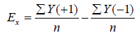 (1)
(1)

Figure 1: A typical chromatogram for a reference solution obtained at nominal conditions.

Figure 2: Represented chromatograms for selected runs of PBD.
Where, Ex is the effect of variable X; ƩY(+1) and ƩY(-1) are the sums of the responses where variable X was at level (+1) and at level (-1), respectively and n is the number of runs in which X was at level (+1) or at level (-1), usually equal to N/2 with N, the number of design experiments.
Analysis of Variance (ANOVA)
The significant effects of each variable on the studied responses were interpreted with the aid of analysis of variance (ANOVA) [5,8]. The sum of squares (SS)X for a variable can be calculated as [ExN/2]2/N while total error is estimated from the sum of the sums of squares from the dummies. The mean square for a variable, (MS)X is obtained from the ratio of (SS)X and the degrees of freedom (df). The F ratio is calculated by dividing (MS)X by (MS)total error and the P value gives an indication of the significance of an effect because it represents the probability of being wrong when accepting that an effect is significant. For example, if the P value is below the considered level of confidence α, an effect may be considered to be statistically significant. For example, when P<0.01 then an effect is significant at α �??0.01.
Table 6 features the effects of the different variables on the considered responses. The variables having a statistically significant effect on a response, at significance levels of 5% (P, 0.05) and of 10% (P, 0.1), were indicated in Table 7. It is clear that none of the variables has a significant effect on the determination of the recovery of the four compounds, whose ranges from Table 5 were narrow and with small percent relative standard deviations (1.1%, 1.4% 1.7% and 1.5% for HCT, OLM, PRL and AMD respectively). Based on these facts, the method for assay of Triolmezest and Inderal tablets can be considered robust as regards recoveries. However, the factorial effects on the other responses that demonstrate the method performance under the different design conditions evidenced that several effects are significant (Table 6). The responses, Rs(OLM-HCT), Rs(PRL-OLM), and Asf(PRL) are affected by most of the tested variables. From Table 6, it was also evidenced that none of the variables could affect Rs(AMDPRL) and was excluded for further study.
| Responses | Variables | ||||||||||
|---|---|---|---|---|---|---|---|---|---|---|---|
| Flow rate | Dum1 | pH | Dum2 | %B start | %B end | Dum3 | Buffer conc | %TEA | Wave length | Dum4 | |
| %HTC | +0.22 | - | +0.65 | -0.46 | -0.52 | - | +0.33 | - | -0.44 | - | - |
| %OLM | - | -0.91 | - | +0.46 | -0.47 | +0.51 | - | -0.36 | +0.26 | +0.50 | -0.23 |
| %PRL | - | - | - | - | - | +1.02 | +0.84 | - | - | -0.83 | - |
| %AMD | +0.48 | -0.81 | +0.32 | -0.049 | - | +0.27 | +0.39 | +0.16 | +0.24 | -0.097 | -0.96 |
| Rs(OLM-HCT) | -0.35 | - | -0.25 | -0.27 | -0.20 | -1.08 | -0.12 | +0.020 | -0.16 | +0.43 | -0.14 |
| Rs(PRL-OLM) | -0.69 | +0.15 | +1.49 | - | +0.63 | +0.63 | -0.13 | +0.73 | +0.41 | -0.20 | -0.57 |
| Rs(AMD-PRL) | - | - | - | - | - | - | -1.10 | - | - | - | - |
| Asf(PRL) | -0.29 | - | -0.14 | +0.22 | +0.14 | +0.23 | +0.028 | +0.16 | -0.44 | -0.24 | +0.16 |
| Asf(AMD) | - | - | -0.39 | +0.42 | +0.36 | - | - | +0.39 | - | +0.39 | - |
| tR(AMD) | -0.67 | - | +0.45 | -0.33 | +0.51 | - | -0.34 | - | +0.62 | -0.67 | - |
Insignificant terms were excluded.
Table 6: Comparison of levels of liver and kidney function at the beginning and end with flaxseed.
| Responses | Variables | ||||||
|---|---|---|---|---|---|---|---|
| Flow rate | pH | %B start | %B end | Buffer conc. | %TEA | Wave length | |
| Rs(OLM-HCT) | **0.0024 | **0.0034 | **0.0042 | **0.0008 | **0.0420 | **0.0053 | **0.0020 |
| Rs(PRL-OLM) | **0.0166 | **0.0078 | **0.0185 | **0.0182 | **0.0159 | **0.0285 | *0.0568 |
| Asf(PRL) | **0.0054 | **0.0117 | **0.0116 | **0.0069 | **0.0102 | **0.0036 | **0.0065 |
| Asf(AMD) | - | *0.0505 | *0.0650 | - | **0.0473 | - | **0.0486 |
| tR(AMD) | **0.0082 | **0.0296 | **0.0202 | - | - | **0.0107 | **0.0079 |
**=Significance at α=0.10 level, *=significance at α=0.05 level.
Table 7: P values obtained for these effects.
Finding the worst-case variable level combinations
It is worth noticing that a statistical significant effect on a response is not always chromatographically relevant; to assess this relevance, the most extreme results from the design experiments have to be considered and compared with the existing SST limits. The most extreme resolution of 1.857 (OLM-HCT) and 1.131 (PRL-OLM); tailing factor of 2.640 (PRL) and 2.785 (AMD) from the design results are not within the SST specifications, namely below 3.671, 2.821; and above 2.624, 2.350 respectively. However, the most extreme design results are not necessarily the worst results since these could be given by a combination of variables not necessarily executed in the design.
To decide on the conditions of this worst-case experiment only the statistically significant effect on a response, at significance levels of 5% (P, 0.05) and of 10% (P, 0.1), were considered. These variables were included because they are able to cause a systematic change in a response when changed from one level to the other. The variables with a P>0.1 were considered as negligible and related only to experimental error. As the PBD is a saturated two-level design, it can only account for linear effects in the prediction of the worst-case situation. This is acceptable because in robustness testing the domain is restricted and only linear effects are important. The variable level combination leading to the worst result for a response Y is predicted by the equation [11]:
Y=EF1F1+EF2F2...............EFKFK (2)
EF1 represents the effect of the variable considered for the worst-case experiment and Fi the level of this variable. Non-important variables (P>0.1) are kept at nominal value. Table 8 details the worst-case variable-level combinations for the different responses. The worst-case experiment was run in triplicate and the mean result was then compared with the system suitability limit by a one-sided t-testto find out if the system suitability limit is statistically violated. Table 9 illustrates the results of the worst-case experiments for the different responses and of the t-tests. Figure 3 depicts the resultant chromatograms for the worst-case experiments. For the resolution (PRL-OLM), the worst case results are not significantly smaller than the SST limit at nominal condition (H1:Rs(PRL-OLM)=3.670>H0:Rs(PRL-OLM)=2.821). The tailing factors are not found to be significantly larger than the limit at nominal condition (H1: Asf (PRL)=1.823<H0:Asf(PRL)=2.624; H1:Asf (AMD)=1.754<H0:Asf(PRL)=2.350).

Figure 3: Chromatograms from the worst-case experiments.
| Responses | Variables | ||||||
|---|---|---|---|---|---|---|---|
| Flow rate | pH | %B start | %B end | Buffer conc | %TEA | Wave length | |
| Rs(OLM-HCT) | +1 (0.9) | +1 (7.3) | +1 (43) | +1 (42) | -1 (18) | +1 (0.5) | -1 (267) |
| Rs(PRL-OLM) | +1 (0.9) | -1 (6.7) | -1 (41) | -1 (38) | -1 (18) | -1 (0.3) | +1 (277) |
| Asf(PRL) | -1 (0.7) | -1 (6.7) | +1 (43) | +1 (42) | +1 (22) | -1 (0.3) | -1 (267) |
| Asf(AMD) | 0 (0.8) | -1 (6.7) | +1 (43) | 0 (40) | +1 (22) | 0 (0.4) | +1 (277) |
| tR(AMD) | +1 (0.9) | -1 (6.7) | -1 (41) | 0 (40) | 0 (20) | -1 (0.3) | +1 (277) |
Table 8: Predicted worst-case variable-level combinations for the different responses.
| Run | Rs(OLM-HCT) | Rs(PRL-OLM) | Asf(PRL) | Asf(AMD) | tR(AMD), min |
|---|---|---|---|---|---|
| 1 | 1.993 | 3.804 | 1.818 | 1.736 | 4.927 |
| 2 | 2.073 | 3.767 | 1.799 | 1.728 | 4.767 |
| 3 | 1.990 | 3.702 | 1.804 | 1.748 | 4.828 |
| Mean | 2.018 | 3.757 | 1.807 | 1.7373 | 4.8406 |
| SD | 0.047078 | 0.051 | 0.009849 | 0.01 | 0.080 |
| Normal SST limits | 3.671 | 2.821 | 2.624 | 2.350 | 5.494 |
| SST limits from worst case results | |||||
 |
 |
 |
 |
 |
|
Table 9: Results of the worst-case experiments for the different responses.
However, it is possible that when the method is transferred to another laboratory, some SST criteria may be violated. In our example, it could be the case for the resolution (OLM-HCT) [H1:Rs(OLMHCT)= 1.939<H0:Rs(OLM-HCT)=3.671]. However, results of the robustness test indicate that the method is robust. It follows that a more or less arbitrary selection of system suitability test parameter limits can lead to problems not related to quality and therefore highly undesirable.
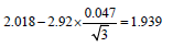
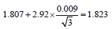
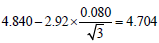
Hence it is better to derive the system suitability limits from the results of the experimental design, as proposed by Mulholland et al. [3,21] who make use of the extreme results to define the SST limits. Since, these extreme results may not be the worst we propose to use the worstcase situations to define the SST limits. This way ambiguous situations may be avoided and SST limits are established, as recommended by the ICH guidelines, from the robustness test. The SST limit could be the upper (for tailing factor) or lower (for resolutions and total analysis time) limit from the one-sided 95% confidence interval [22] around the worst-case mean.
The lower limit is  while the upper one is
 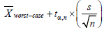 . This would lead to system suitability limits of 1.939 for the Rs(OLM-HCT), 3.670 for the Rs(PRL-OLM), 1.823 for the Asf(PRL), 1.754 for the Asf(AMD), and 4.704 for the total analysis time (Table 9). Noteworthy this approach give some SST limits stricter than the previously used ones [resolution Rs(OLM-HCT)].
The rationale for this approach is beside the recommendation of the ICH guidelines. Defining SST limits on the basis of a robustness test results can be endorsed also for practical reasons. For example, when a separation method was properly optimized, the quantitative results did not change significantly, although some of the SST limits (selected rather arbitrarily and independently from the results of a robustness test) were frequently violated. This may happen if they were set too strictly during method optimization.
Conclusion
The conclusion for the robustness test of the chromatographic method for the analysis of Triolmezest and Inderal film-coated tablets is that the method is robust concerning the analysis results of the four compounds.
Defining system suitability limits based on the worst-case results for which the conditions were predicted from the robustness test, allows to avoid an undesirable situation where a method is found to be robust for its quantitative aspect while some externally defined system suitability criteria are violated.
References
- ICH Harmonized Tripartite Guideline Q2(R1) (2005) Validation of Analytical Procedures: Text and Methodology, International Conference on Harmonisation of Technical Requirements for registration of Pharmaceuticals for Human Use.
- Youden WJ, Steiner EH (1975) Statistical manual of the Association of Official Analytical Chemists; Statistical techniques for collaborative tests, planning and analysis of results of collaborative tests. p: 96.
- Mulholland M (1988) Ruggedness testing in analytical chemistry. Trends Anal Chem 7: 383-389.
- Van Leeuwen JA, Buydens LMC, Vandeginste BGM, Kateman G, Schoenmakers PJ, et al. (1991) RES, an expert system for the set-up and interpretation of a ruggedness test in HPLC method validation. Part 1: The ruggedness test in HPLC method validation.ChemometIntell Lab Systems 10: 337-347.
- Heyden YV, Massart DL (1996) Robustness of Analytical Methods and Pharmaceutical Technological Products. Elsevier, Amsterdam, pp: 79-147.
- Jimidar M, Niemeijer N, Peeters R, Hoogmartens J (1998) Robustness testing of a liquid chromatography method for the determination of vorozole and its related compounds in oral tablets. J Pharm Biomed Anal 18: 479-485.
- Plackett RL, Burman JP (1946) The design of optimum multifactorial experiments.Biometrika 33: 305-325.
- Morgan E (1991) Chemometrics-Experimental Design. Analytical Chemistry by Open Learning. Wiley, Chichester.
- Jimidar M, Khots MS, Hamoir TP, Massart DL (1993) Application of a fractional factorial experimental design for the optimization of fluoride and phosphate separation in capillary zone electrophoresis with indirect photometric detection.Quim Anal 12: 63-68.
- Dejaegher B, Dumarey M, Capron X, Bloomfield MS, Heyden YV (2007) Comparison of Plackett��?Burman and supersaturated designs in robustness testing. Anal Chim Acta 595: 59-71.
- Heyden YV, Jimidar M, Hund E, Niemeijer N, Peeters R, et al. (1999) Determination of system suitability limits with a robustness test. J Chromatogr A 845: 145-154.
- Heyden YV, Nijhuis A, Smeyers-Verbeke J, Vandeginste BGM, Massart DL (2001) Guidance for robustness/ruggedness tests in method validation. J Pharm Biomed Anal 24: 723-753.
- Levine CB, Fahrbach KR, Frame D, Connelly JE, Estok RP, et al. (2003) Effect of amlodipine on systolic blood pressure. ClinTher 25: 35-57.
- Liew D, Liu L, Jeffers BW, Foody J (2014) PW177 Literature review of the cost and cost effectiveness of amlodipine in the treatment of hypertension. Glob Heart 9: e293-e294.
- Dubey N, Jain A, Raghuwanshi AK, Jain DK (2012) Simultaneous Determination and Validation of OlmesartanMedoxomil, Amlodipine Besilate and Hydrochlorothiazide in Combined Tablet Dosage Form Using RP-HPLC Method. Asian J Chem 24: 4535-4537.
- da Silva Sangoi M, Wrasse-Sangoi M, de Oliveira PR, Todeschini V, Rolim CMB (2011) Rapid simultaneous determination of aliskiren and hydrochlorothiazide from their pharmaceutical formulations by monolithic silica HPLC column employing experimental designs. J LiqChromRelTechnol 34: 1976-1996.
- Li H, Wang Y, Jiang Y, Tang Y, Wang J, et al. (2007) A liquid chromatography/tandem mass spectrometry method for the simultaneous quantification of valsartan and hydrochlorothiazide in human plasma. J Chromatogr B 852: 436-442.
- Vignaduzzo SE, Castellano PM, Kaufman TS (2011) Development and validation of an HPLC method for the simultaneous determination of amlodipine, hydrochlorothiazide, and valsartan in tablets of their novel triple combination and binary pharmaceutical associations.J LiqChromRelTechnol 34: 2383-2395.
- Sharma M, Kothari C, Sherikar O, Mehta P (2014) Concurrent Estimation of Amlodipine Besylate, Hydrochlorothiazide and Valsartan by RP-HPLC, HPTLC and UV��?Spectrophotometry. J Chromatogr Sci 52: 27-35.
- Hemke AT, Bhure MV, Chouhan KS, Gupta KR, Wadodkar SG (2010) UV Spectrophotometric Determination of Hydrochlorothiazide and OlmesartanMedoxomil in Pharmaceutical Formulation. J Chem 7: 1156-1161.
- Mulholland M, Waterhouse J (1987) Development and evaluation of an automated procedure for the ruggedness testing of chromatographic conditions in high-performance liquid chromatography, J Chromatogr A 395: 539-551.
- Massart DL, Vandeginste BGM, Buydens LMC, De Jong S, Lewi PJ, et al.(1997) Handbook of Chemometrics and Qualimetrics- Part A. Elsevier, Amsterdam.
Relevant Topics
Recommended Journals
Article Tools
Article Usage
- Total views: 10451
- [From(publication date):
June-2017 - Jul 04, 2025] - Breakdown by view type
- HTML page views : 9338
- PDF downloads : 1113