Research Article Open Access
Climate Modeling of Jhelum River Basin - A Comparative Study
Mehnaza Akhter* and Ahanger Manzoor Ahmad
Department of Civil Engineering, NIT Srinagar, J&K, India
- *Corresponding Author:
- Mehnaza Akhter
Department of Civil Engineering
NIT Srinagar,J&K, India
Tel: 9622927355
E-mail: mehnaz9jun@yahoo.com
Received date: December 05, 2016; Accepted date: January 23, 2017; Published date: January 30, 2017
Citation: Mehnaza Akhter, Ahanger Manzoor Ahmad (2017) Climate Modeling of Jhelum River Basin - A Comparative Study. Environ Pollut Climate Change 1:110.
Copyright: © 2017 Akhter M, et al. This is an open-access article distributed under the terms of the Creative Commons Attribution License, which permits unrestricted use, distribution, and reproduction in any medium, provided the original author and source are credited.
Visit for more related articles at Environment Pollution and Climate Change
Abstract
Global Circulation Models (GCMs) are a major tool used for future projections of climate change using different emission scenarios. However, for assessing the hydrological impacts of climate change at regional scale, the GCM outputs cannot be used directly due to the mismatch in the spatial resolution between the GCMs and hydrological models. In order to use the output of a GCM for conducting hydrological impact studies, downscaling is used. Among the variables usually downscaled, precipitation and temperature downscaling is quite challenging and is more prone to uncertainty issues than other climatological variables. The downscaling methods used for this study belong to the following downscaling categories; (1) Multiple linear regression; and (2) Artificial neural network. In this study the future projections of climate were made under A1B scenario up to 21st century using CGCM3 model. At the end of the 21st century the mean annual temperature of the Jhelum river basin is predicted to increase by 2.36°C and 1.43°C under A1B scenario using MLR and ANN technique respectively whereas the total annual precipitation is predicted to decrease substantially by 36.53% and 30.88% under A1B scenario by MLR and ANN technique, respectively.
Keywords
Downscaling; ANN; MLR; Climate change; Temperature; Precipitation; Jhelum river basin; SRES A1B and A2 scenarios.
Introduction
Industrialization and urbanization are increasing dramatically, along with population growth all over the world. Increased emission of greenhouse gases, especially CO2 causes global warming. The global and regional climate has been changing as evidenced by increases in temperature and rainfall intensity. The impacts of climate change; primarily driven by global warming, are highly extensive, complicated and uncertain. Global surface temperature has risen by 0.74°C during the twentieth century and the warming trend has accelerated in the last 50 years [1]. Climate change impacts, such as changes in precipitation and temperature, are leading to more floods and drought events each year. Climate variability and change has a huge effect on the general well-being of communities across the world, and many living organisms are sensitive to changing climate patterns. Availability and variability of water resources have been affected by climate change effects. Climate change has affected water resources globally and regionally in the last 30 years. In Particular, rainfall, known as the main driver of hydrological cycle, has been varying in most parts of the world. The change in climate variables such as rainfall and temperature has redistributed the public health, industrial, irrigation, and municipal water demands and the ecosystem [2].Climate change is threatening the socio-economic development of Kashmir valley. The study area, Jhelum River is a major tributary of river Chenab. The precipitation and river flow in the Jhelum River Basin have changed, resulting in floods and droughts in this basin because of climate change impacts. Consequently, floods and droughts have caused degradation of natural water resources [3]. It was reported that annual rainfall has decreased and seasonal inflow to this basin was also reduced during the summer season. In summer, many areas in the Jhelum River Basin are known for their scanty annual rainfall, very high rates of evaporation and consequent insufficiency in renewable water resources, and reduced water storage capacity. Water yields decline at the basin outlet during the summer and winter but increase during the rainy season. The outflow from this basin is insufficient for the downstream area. On the other hand, there are also serious floods in the Jhelum River Basin because of heavy precipitation in very short duration in mostly upper reaches of the basin. Hence to predict the future climate of basin downscaling is used.
Two downscaling approaches that are commonly used are statistical downscaling and dynamical downscaling. Statistical downscaling assumes that relationships between large scale and local climate are constant. It combines GCM output with local observations in order to obtain their statistical relationships. Local climate forecast can then be determined from such relationships. Dynamical downscaling involves nesting regional climate model into an existing global climate model. Numerical meteorological modeling is used in dynamical downscaling approach.
Various methods have been employed to derive relationships in statistical downscaling to forecast different climate information in different parts of the world. Such methods include canonical correlation analysis, multiple linear regressions, artificial neural networks and support vector machine. The rest of this section summarizes some previous studies on statistical downscaling methods.
Htut et al. [4] aimed to forecast the climate change scenarios of Bago River Basin in Myanmar. A delta change method was used to correct the bias of maximum and minimum temperature and precipitation. It was observed that average annual maximum and minimum temperatures are projected to rise in the entire basin most significantly in the 2080s. Average annual precipitation shows a distinct increase in the 21st century with the greatest upturn in the 2050s.
Shashikanth et al. [5] used a kernel based approach on the CMIP5 GCM data set to derive the Indian summer monsoon rainfall on a fine scale of 25 Km. The downscaling technique consisted of two steps: the derivation of rainfall state using the Classification and Regression Tree (CART) and then estimation of rainfall using kernel regression (KR) estimator on a daily time step. One of the most recent studies in daily downscaling has been conducted in Kannan et al. [6], where non-parametric kernel regression model was used for downscaling of multisite daily precipitation. The simulation of rainfall state was done for the entire study area from large scale atmospheric variables using the CART algorithm and then the result was projected as a rainfall estimator. The paper concludes that the south of the Mahanadi basin shows an increasing trend whereas the northern part of the basin shows a decreasing trend.
Fiseha et al. [7] Two statistical downscaling techniques, namely regression based downscaling and the stochastic weather generator, were used to downscale the HadCM3, GCM predictions of the A2 and B2 scenarios for the Upper Tiber River basin located in central Italy. The Statistical Downscaling Model (SDSM) based downscaling shows an increasing trend in both minimum and maximum temperature as well as precipitation in the study area until the end of the 2080s. Long Ashton Research Station Weather Generator (LARS-WG) shows an agreement with SDSM for temperature, however, the precipitation shows a decreasing trend with a pronounced decrease of summer season that goes up to 60% in the time window of the 2080s as compared to the current (1961-1990) climate.
Aksornsingchai et al. [8] have explored three statistical techniques to predict both rainfall and temperature using multiple linear regression (MLR), support vector machine with polynomial kernel and support vector machine with radial basis function. Five predictands namely; temperature, pressure, precipitation, evaporator and net short wave radiation were selected for the study.
Wilby et al. [9] reported the use of weather generator and ANN as transfer functions. The weather generator performed better while simulating spell-length events and their duration. The weather generator’s result shows only a small difference between the observed and the simulated precipitation. ANN seemed to perform poorly because of its inability to simulate the dry-wet occurrences well. Its poor performance was attributed to the model’s tendency to produce many “wet days”.
Wilby et al. [10] analyzed the correlation between the predictor and predictand and selected the predictors that explained the high variance in the precipitation occurrence. These selected predictors were then used to downscale the GCM to get daily precipitation.
The Special Report on Emission Scenarios (SRES) establishes different future world development possibilities in the 21st century, taking into consideration the possible changes in various factors including economic development, technological development, energy intensities, energy demand, and structure of energy use, resources availability, population change and land-use change. The possibilities of changes in future developments are categorized mainly in the form of four major storylines quantified as four scenarios namely A1, A2, B1 and B2. The scenarios include the expected range of emissions of greenhouse gases (GHGs), sulphur and their respective driving forces. Family A1 assumes rapid economic and population growth which peaks mid century and declines thereafter. The B designation represents a more balanced shift between fossil fuel and alternative energy sources.
In the present study the multiple linear regressions and artificial neural network technique was employed to relate the GCM predictors with the predictands, such as the locally observed precipitation and temperature at four meteorological observatories namely Srinagar, Pahalgam, Qazigund and Gulmarg of Jhelum river basin which is located in the state of Jammu and Kashmir, India. The predictors were obtained from Canadian third generation Climate model (CGCM3).
| S. No. | Station name | Latitude (°N) | Longitude (°E) | Elevation (m a.s.l) |
|---|---|---|---|---|
| 1 | Srinagar | 34.09 | 74.79 | 560 |
| 2 | Qazigund | 33.63 | 75.15 | 1670 |
| 3 | Pahalgam | 34.01 | 75.19 | 2740 |
| 4 | Gulmarg | 34.15 | 74.25 | 2690 |
Table 1: List of stations incorporated in the study, with location and elevation information.
Study Area and Data Description
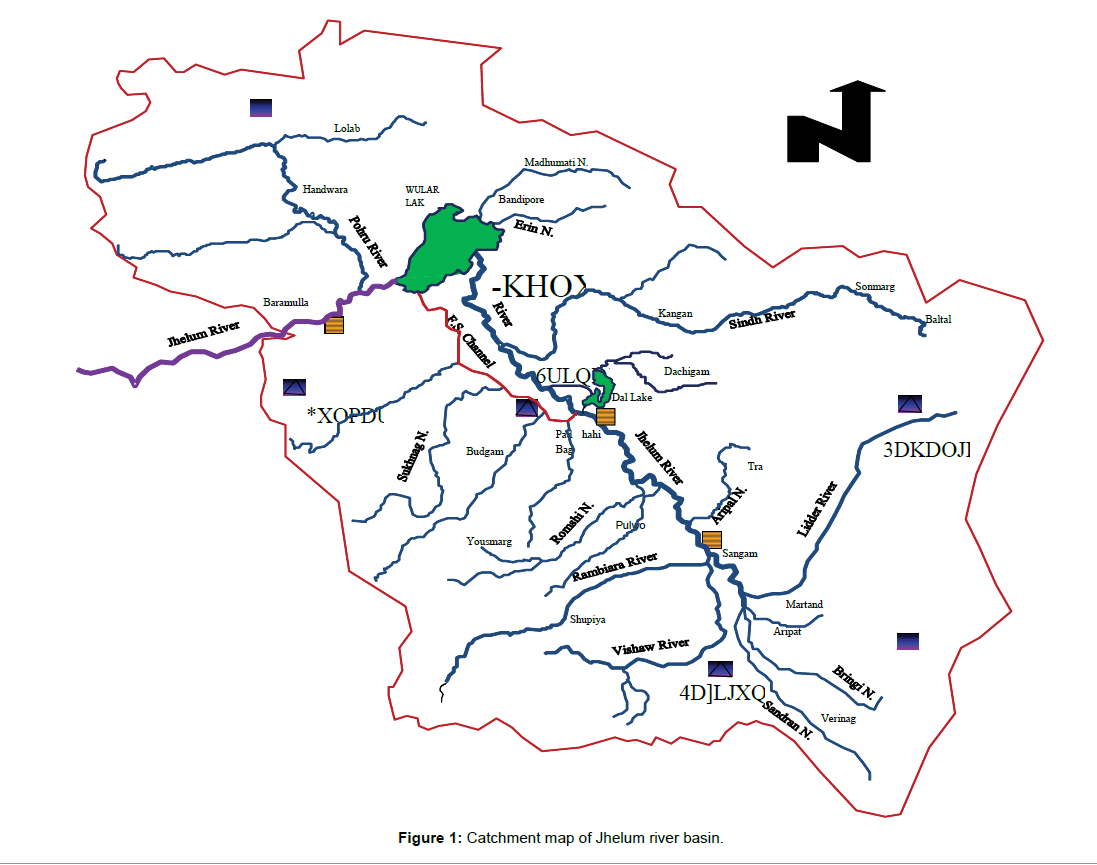
The catchment of the Jhelum River lies between 33°25’ N to 34°40’ N latitude and 73°55’ E to 75°35’E longitude. River Jhelum is a major tributary of river Chenab which itself is a tributary of river Indus. The study area comprises of the Jhelum basin located in the state of Jammu and Kashmir, India. The total geographical area of Jhelum basin up to Indo-Pakistan border is about 17622 Sq. Km with the main channel length of 165 Km. The average elevation of Jhelum basin is about 1830 metres above mean sea level. It originates from the Verinag’s spring in the north-west side of Pir Panjal and moves parallel to the Indus River at an average elevation of 5,500 ft. It moves through the area of about 2300 mile2 alluvial soil of Kashmir Valley. On the North side of Kashmir valley, there are large sources of glaciers which also contribute to Jhelum River. Moving towards north-west direction and after flowing through the Srinagar, which is the capital of Jammu and Kashmir, it joins the Dal and Wular lakes near Baramulla where it drops coarse sediments. Leaving the Baramulla, it flows through a long gorge of 80 miles with mean slope of 33 feet per mile. It ends in a confluence with the Chenab. Near Muzaffarabad, a biggest tributary of Jhelum River called as Kishanganga (Nelum) joins it at the place of Domel. It covers almost all the physiographic divisions of the Kashmir Valley and is drained by the most important tributaries of river Jhelum. Srinagar city which is the largest urban centre in the valley is settled on both the sides of River Jhelum and is experiencing a fast spatial growth. Figure 1 shows the catchment map of river Jhelum and locations of four National Meteorological Observatory (NMO) stations namely Srinagar, Qazigund, Pahalgam and Gulmarg selected for the study.
Data description
Station data: Historical observed monthly data of mean temperature and precipitation are collected from India Meteorological Department (IMD), Pune and NCDC (national climate data centre) website for four National Meteorological Observatory (NMO) stations namely Srinagar, Qazigund, Pahalgam, and Gulmarg (Table 1) for the period 1979 to 2013.
GCM data: GCM data was downloaded from the CCDS portal, i.e., Canadian Climate Data and Scenarios (CCDS) website http:// ccds-dscc.ec.gc.ca/ and http://www.cccsn.ec.gc.ca/. CGCM3 model was selected for the study; and A1B scenario was selected on the basis of literature review.
The input variables include the following GCM predictors:
1. Tempas (mean temperature at 2 m)
2. Mslpas (mean sea level pressure),
3. Humas (specific humidity at 2 m),
4. Relative humidity (rhum),
5. Zonal velocity component (u),
6. Meridional velocity component (v)
The GCM predictors of tempas, u, v and rhum were found to be most appropriate independent variables for temperature and those of tempas, humas, mslpas and u for precipitation after p-test analysis.
Methodology
Multiple linear regression analysis technique
In the present study the multiple linear regression technique was employed to relate the GCM predictors with the predictands such as the locally observed precipitation and temperature at four meteorological observatories namely Srinagar, Pahalgam, Qazigund and Gulmarg of Kashmir valley India. Minitab 15.0 statistical software was also used for regression analysis in addition to MS-Excel. The large scale GCM predictors were related to locally observed precipitation and temperature.
Multiple linear regression analysis was performed using MS-Excel Data Analysis Tool Pack and Minitab 15.0 Statistical Tool Pack. The best fit is calculated for the given dataset. The regression model used for prediction is given in Eq. 3.1.

Where, y is the dependent (or response) variable, x is independent (or predictor) variable and Æ is the error term. The intercept and the regression coefficients were obtained using Minitab software.
Matlab: Neural network toolbox
ANN has gained wide recognition due to its capability to simulate and estimate non-linear relationships well. Hewitson et al. [11] established a mathematical relationship between long term observational data and the atmospheric circulation variables using Artificial Neural Network (ANN), since it removes the problem of categorizing the circulation features and their characteristics. The study indicated that ANN captures non-linear aspects of the predictorpredictand relationship effectively. ANN was seen to be more robust than linear regression methods.
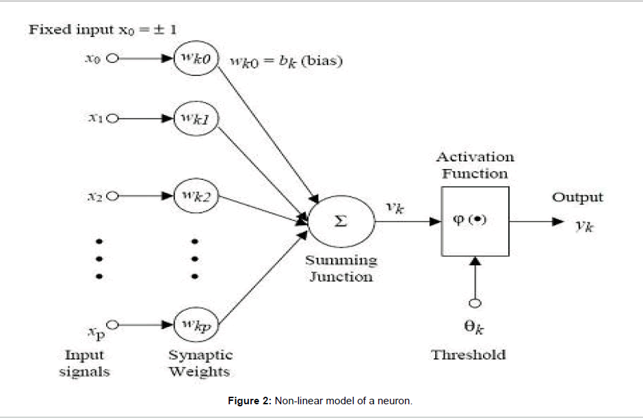
Neural Networks are simplified models of biological neuron system. A neural network is a massively parallel distributed processor made up of simple processing units, which has a natural propensity for storing experiential knowledge and making it available for use .The fundamental processing element of an ANN is an artificial neuron. Just like the natural neuron in human brain, it can receive inputs, process them and produce the relevant output. A simple mathematical model in Figure 2 can be used in explaining a neuron quantitatively. The three basic elements of the neuronal model are: a set of synapses or connecting links, an adder and an activation function. This model also includes an externally applied bias, denoted by bk.
A network of neurons is formed when a neuron links with others via synapses which can be single layered or multi layered. A multilayer ANN contains an input layer of neurons, an output layer of neurons, and one or more hidden layer of neurons. The hidden layer aids in performing useful intermediary computations before directing the input to the output layer.
When a network had been constructed for a specific application, inputs and the corresponding targets are used to train a network until it learns to associate a particular input with a reasonable output. A network is ideally trained until the change in weights in a training cycle reaches a minimum value. After the network is properly trained, it has to be tested for its ability to produce accurate outputs. Large multilayered networks with multiple nodes in each layer are capable of memorizing data due to the vast number of synaptic weights available on such a network. Thus, generating correct outputs for input vectors encountered within the training process does not justify the ability of a network to generate accurate outputs.
Among the different types of neural networks, those which are mostly concentrated in this research work are Rosenblatt’s perceptrons, also known as multilayer feed-forward neural networks. In these nets there is a layer of input units whose only role is to feed input patterns into the rest of the network. Next, there are one or more intermediate or hidden layers of neurons evaluating the same kind of function of the weighted sum of inputs, which, in turn, send it forward to units in the following layer. This process goes on until the final or output level is reached, thus making it possible to read off the computation.
In this paper, two observed data have been used for MLR and ANN model, which are rainfall and temperature. Performance of MLR and ANN model is measured using coefficient of determination (R2), root mean square error coefficient (RMSE) and mean absolute deviation (MAD).
Results and Discussion
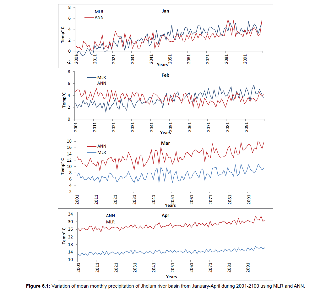
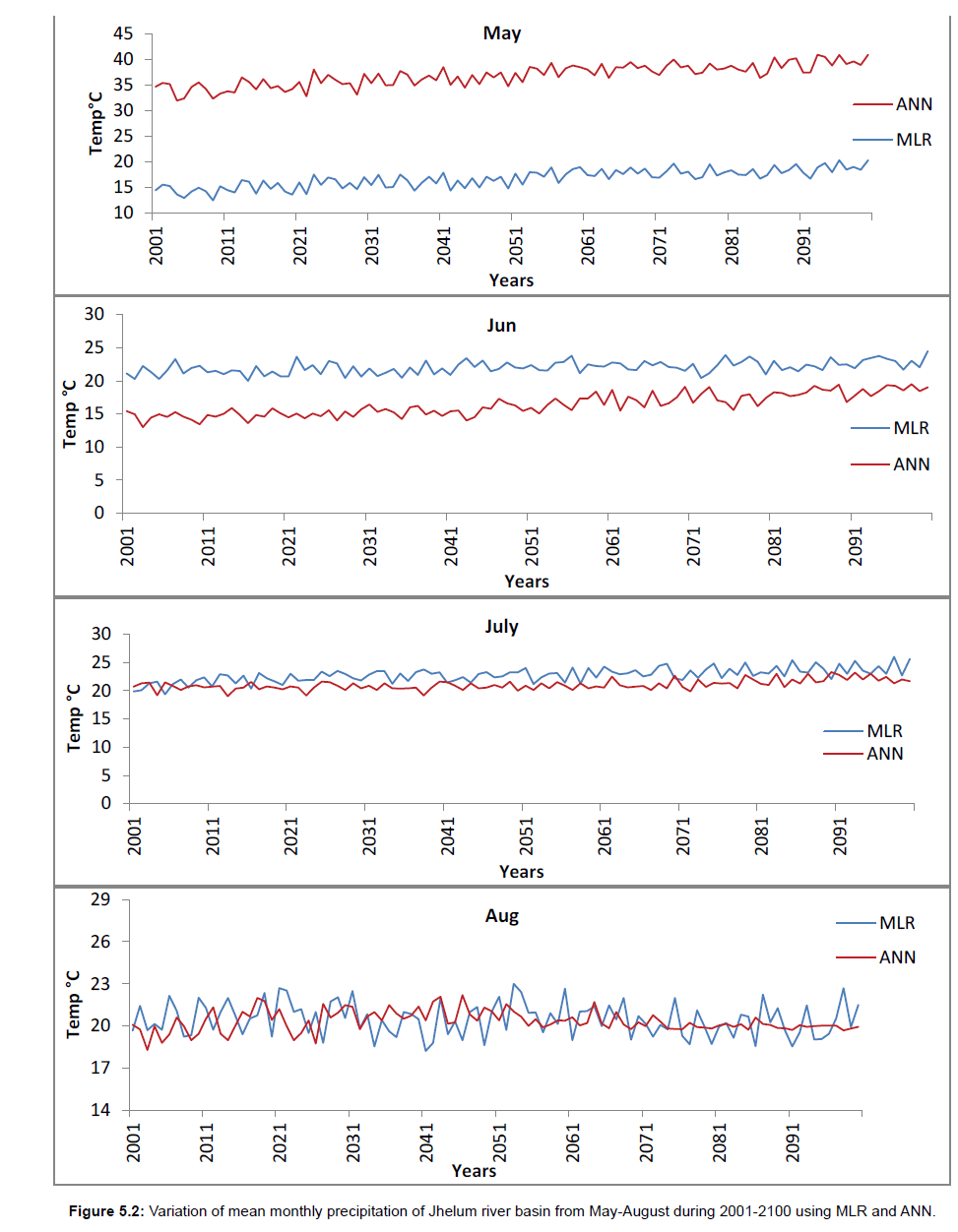
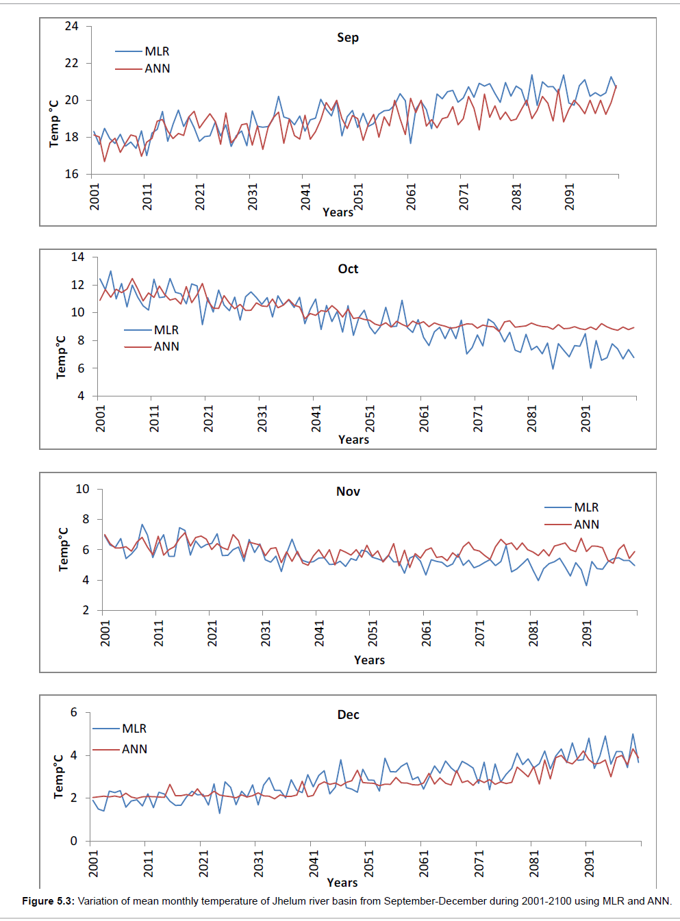
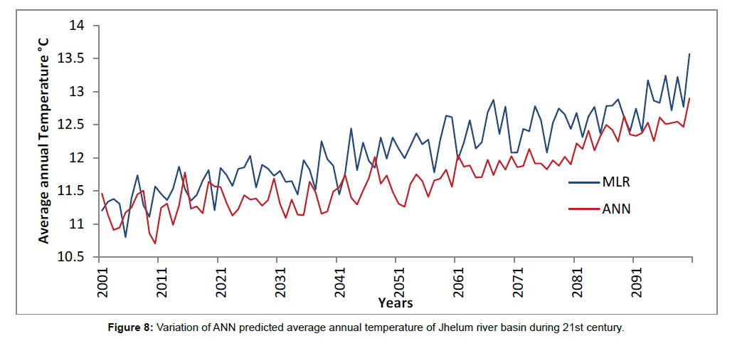
The MLR and ANN models were operated for mean monthly temperature and monthly rainfall of Jhelum river basin. The regression model was validated on the observed data of mean monthly temperature and precipitation for the period 2010-2013. The regression statistics for temperature and precipitation are given in Tables 2 and 3. Figure 3 shows the validation of temperature model and Figure 4 shows the validation of precipitation model over the period 2010 to 2013. From Figure 3 it is clear that the observed and predicted values of temperature varied in the same direction throughout the validation period. Furthermore, the future mean monthly temperatures of the Jhelum basin for the period 2001-2100 were predicted by MLR and ANN models and are shown in Figures 5.1-5.3. The average annual temperature of Jhelum basin at the end of the 21st century was also predicted using MLR and ANN models and was found to increase by 2.36°C and 1.43°C, respectively under A1B scenario.
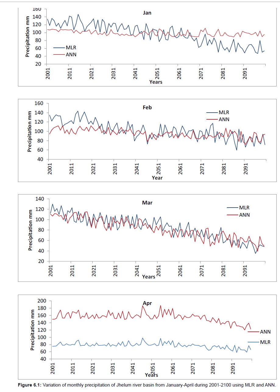
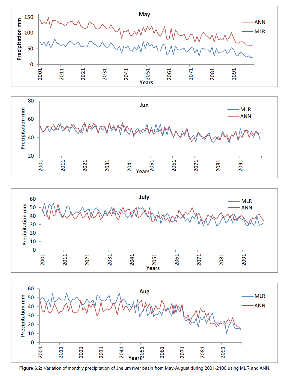
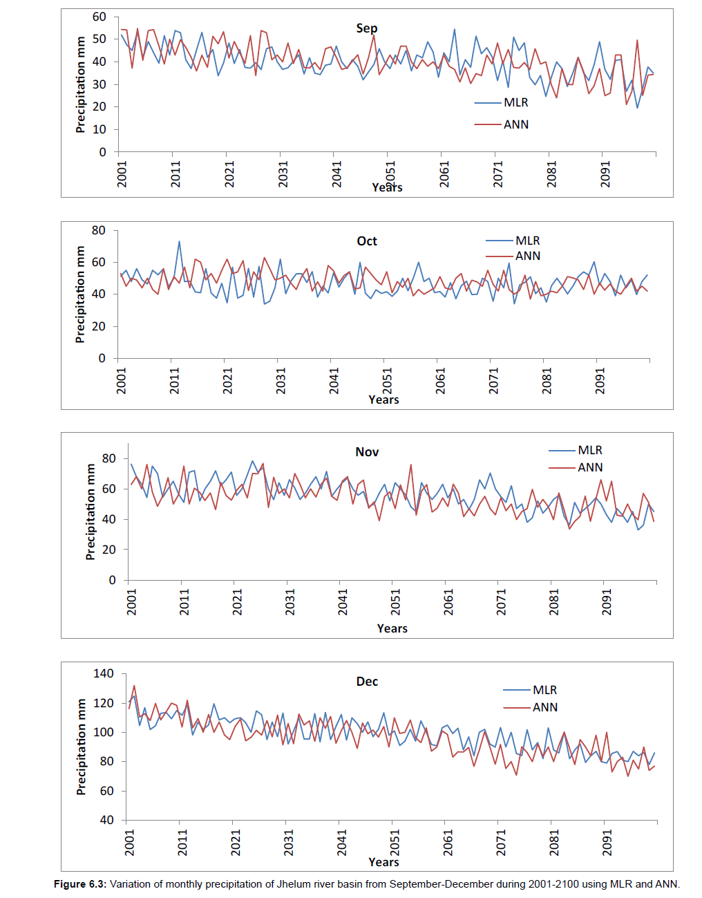
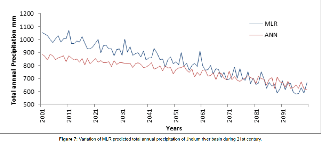
Similarly the future monthly precipitation of the Jhelum basin for the period 2001-2100 were predicted by MLR and ANN models and are shown in Figures 6.1-6.3.It was observed that the mean monthly precipitation of Jhelum basin is expected to decrease continuously over the 21st century. This decrease in monthly total precipitation is more pronounced from December to April, the major precipitation season of the basin. The total annual precipitation of Jhelum basin during the period 2001-2100 was also predicted using MLR and ANN models. Figure 7 represents the variation of this annual precipitation over a 100 year period of 2001-2100 and shows that annual precipitation is expected to decrease by about by 36.53% and 30.88% under A1B scenario by MLR and ANN technique respectively.
| Month | Regression Equation using MLR and Minitab | R2 |
|---|---|---|
| Jan | Y=-3.080+1.364X1+0.101X2-1.355X3+0.434X4 | 0.92 |
| Feb | Y=3.880+0.678X1-2.61X2-2.04X3+0.11X4 | 0.79 |
| Mar | Y=7.661+0.75X1+5.38X2-5.720X3+0.054X4 | 0.86 |
| Apr | Y=9.59-0.13X1+2.77X2+0.103X3-0.078X4 | 0.78 |
| May | Y=13.60 -0.56 X1-1.70X2-0.86 X3+0.276 X4 | 0.74 |
| Jun | Y=14.46+0.198 X1-0.61 X2-0.65 X3+0.03X4 | 0.67 |
| July | Y=20.0-0.25 X1+1.98 X2-3.27 X3+0.10 X4 | 0.87 |
| Aug | Y=21.46+1.02X1+0.45 X2+1.66 X3-0.40 X4 | 0.65 |
| Sep | Y=10.93+0.41 X1+0.48X2-0.57X3-0.05 X4 | 0.73 |
| Oct | Y=9.55-1.24X1+2.58X2-4.90X3+0.14X4 | 0.81 |
| Nov | Y=6.32-0.65X1-2.79 X2-1.05X3+0.022X4 | 0.90 |
| Dec | Y=2.89+0.61 X1-0.91X2-0.18X3+0.096 X4 | 0.80 |
| Mean temperature predictors: Tempas (mean temp at 2m) X1, zonal velocity (u) X2, meridional velocity (v) X3, relative humidity(rhum) X4 | ||
Table 2: Regression equations for temperature using MLR from the period 1979-2013 for CGCM3.
| Month | Regression Equation using MLR and Minitab | R2 |
|---|---|---|
| Jan | Y=588.28+14.9X1-0.346X2+0.45X3+5.01X4 | 0.57 |
| Feb | Y=8703-2.64X1-0.79X2-8.64X3+6.31X4 | 0.74 |
| Mar | Y=-7339.78-0.59X1-2.2X2+1.73X3-0.08X4 | 0.66 |
| Apr | Y=-20082.90+1.39X1+2.68X2+7.15X3-2.66X4 | 0.70 |
| May | Y=9164.42 -1.47 X1+3.26X2-9.11X3+2.24X4 | 0.64 |
| Jun | Y=-10586.3+2.48 X1-19.9 X2+0.9 X3-0.64 X4 | 0.77 |
| July | Y=22.8-0.29 X1+2.58 X2-3.04 X3-0.12 X4 | 0.84 |
| Aug | Y=6349.28+6.41X1+6.32 X2+5.99 X3+6.69 X4 | 0.65 |
| Sep | Y=3094.34+12.7 X1+4.26X2+2.99X3+3.3X4 | 0.73 |
| Oct | Y=4057.986-4.05X1-3,87X2+3.29X3-1.15X4 | 0.71 |
| Nov | Y=5905.62-5.28X1+8.4 X2-4.8X3+5.2X4 | 0.67 |
| Dec | Y=128.70-2.79 X1+0.15X2+5.0X3-0.21 X4 | 0.69 |
| Precipitation predictors: Tempas (mean temp at 2m) X1, specific humidity (humas) X2, mean sea level pressure (mslpas) X3,zonal velocity (u) X4 | ||
Table 3: Regression equations for precipitation using MLR from the period 1979-2009 for CGCM3.
The coefficient (R2) for temperature ranges from 0.65-0.92 for the mean ensembles which indicates a strong correlation. However for precipitation it lies in the range of 0.57-0.77 (less than that for temperature).
Regression statistics of both MLR and ANN model was done for validation period 2010-2013 for temperature and precipitation. Results of regression statistics are shown in Tables 4 and 5. From Figures 3 and 4 it is clear that the observed and predicted values of temperature and precipitation were close for ANN technique than MLR throughout the validation period .Thus ANN technique gave better results than MLR revealing that the ANN technique was superior than MLR from the statistical analysis of different parameters.
The downscaled monthly mean temperature shows an increasing trend in all months except for October and November for the period 2001–2100 for A1B scenario by both techniques. In general, the annual mean temperature shows an increasing trend in A1B scenario (Figure 8).The average annual temperature is predicted to increase by 2.36°C and 1.43°C under A1B scenario using MLR and ANN technique respectively over 21st century in Jhelum river basin. Also for the months of April and May mean temperature and precipitation as predicted by MLR and ANN shows large variation because in Jhelum river basin major change in these parameters occurs at the end of March as season changes from winter to summer so the value of input variables varies from one station to another. Besides rainfall is a random phenomenon the intensity of rainfall varies from one place to another at the same time. Hence we observe large variation in climate variables over time by different techniques.
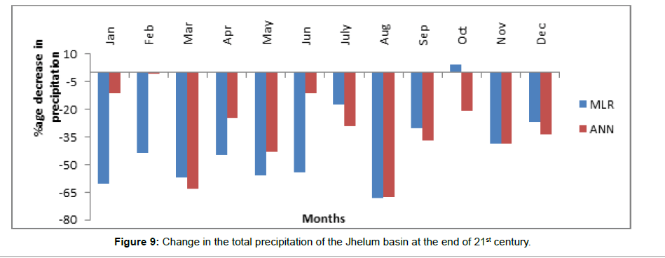
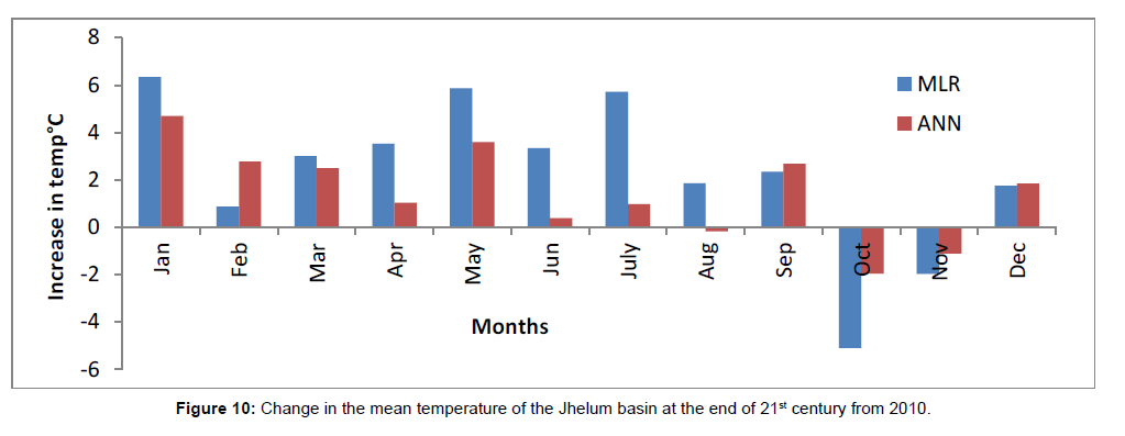
The rainfall amounts generally show a decrease trend throughout the year especially in the month of January and August and a small increase for the month of October for the period 2001–2100 for the CGCM3 model for A1B scenario. The total annual precipitation is predicted to decrease substantially by 36.53% and 30.88% under A1B scenario by MLR and ANN technique respectively over 21st century using CGCM3 model data in the Jhelum river basin (Figures 7, 9 and 10).
Tables 4 and 5 shows the regression statistics values of mean square error (MSE), root mean square error (RMSE) and mean absolute deviation (MAD) of ANN model for validation period of 2010-2013 for temperature and precipitation, respectively. From the statistical parameters of temperature validation using ANN model, value of MSE, RMSE and MAD works out to be least for CGCM3 A1B scenario and more for precipitation validation. Hence temperature is validated to a much higher accuracy than precipitation by climate models.
Conclusion
Results from Minitab were preferred than MS-Excel as the error was less and R2 value was more. Moreover it does filtering of data along with regression. The results from Minitab were transferred to MS-Excel and graphs were plotted in Excel.
From the results of the analysis the following conclusions were drawn:
• Both MLR and ANN models predict an increase in mean monthly temperature of Jhelum river basin over the 21st century. Although the MLR model predicts an increase in mean temperature during all months except for some months such as October and November. ANN predicts more increase in temperature for the months March, April and May than predicted by MLR. The mean annual temperature of the valley is expected to increase by the end of 21st century by both models.
• The mean annual temperature of the Jhelum river basin is predicted to increase by 2.36°C and 1.43°C under A1B scenario using MLR and ANN technique respectively over 21st century.
| Month | MSE | RMSE | MAD |
|---|---|---|---|
| January | 0.001259 | 0.035480 | 0.021521 |
| February | 0.002368 | 0.048658 | 0.025765 |
| March | 0.018746 | 0.136916 | -0.077500 |
| April | 0.003382 | 0.058152 | -0.049690 |
| May | 0.00681 | 0.082525 | -0.023970 |
| June | 0.020214 | 0.142178 | -0.088110 |
| July | 0.044278 | 0.210424 | 0.081197 |
| August | 0.012225 | 0.110567 | -0.047500 |
| September | 0.009688 | 0.098426 | -0.041860 |
| October | 0.008527 | 0.092344 | 0.007558 |
| November | 0.031696 | 0.178033 | -0.072740 |
| December | 0.011327 | 0.106430 | 0.048770 |
Table 4: Statistical parameters of ANN validation for temperature using CGCM3 model for A1B scenario.
| Month | MSE | RMSE | MAD |
|---|---|---|---|
| January | 0.550001 | 0.741620 | -0.85179 |
| February | 0.555556 | 0.745356 | -0.33321 |
| March | 0.558400 | 0.747262 | -0.16000 |
| April | 0.016172 | 0.127170 | -0.10063 |
| May | 0.171383 | 0.413984 | -0.30533 |
| June | 0.474336 | 0.688721 | 0.46576 |
| July | 0.438580 | 0.662254 | 0.41128 |
| August | 0.344438 | 0.586888 | -0.10334 |
| September | 0.550001 | 0.741620 | -0.75236 |
| October | 0.300002 | 0.547724 | 0.01038 |
| November | 0.575100 | 0.758353 | 0.95709 |
| December | 0.400609 | 0.632937 | -0.46965 |
Table 5: Statistical parameters of ANN model validation for precipitation using CGCM3 predictors for A1B scenario.
• The monthly total precipitation of Jhelum river basin was found to decrease by both MLR and ANN models. The MLR model predicted a pronounced decrease in all months except for some months such as July, September and October. For the month of April and May, ANN predicted much more decrease in precipitation than predicted by MLR model.
• The total annual precipitation is predicted to decrease by 36.53% and 30.88% under A1B scenario by MLR and ANN technique respectively in the Jhelum river basin.
• ANN model gave better results than MLR revealing that the ANN technique was superior to MLR from the statistical analysis of different parameters. Also observed temperature and precipitation values for validation period were close to the predicted values using for ANN technique.
References
- IPCC (2007) Climate change 2007: The physical science basis. Contribution of working group I to the fourth assessment report of the intergovernmental panel on climate change. Cambridge University Press, Cambridge, UK.
- Zhang Y, Sun S, Seth C, Manvendra K, He J (2011) CCSM3 simulated regional effects of anthropogenic aerosols for two contrasting scenarios: Rising Asian emissions and global reduction of aerosols. Int J Climatol 31: 95-114.
- Hlaing K, Haruyama S, Aye MM (2008) Using GIS-based distributed soil loss modeling and morphometric analysis to prioritize watershed for soil conservation in Bago river basin of lower Myanmar. Front Earth Sci China 2: 465-478.
- Htut AY, Shrestha S, Nitivattananon V, Kawasaki A (2014) Forecasting climate change scenarios in the Bago river basin, Myanmar. J Earth Sci Clim Change.
- Shashikanth K, Ghosh S (2013) Fine resolution indian summer monsoon rainfall projection with statistical downscaling. IJCEBS 1.
- Kannan S, Ghosh S (2013) A non parametric kernel regression model for downscaling multisite daily precipitation in Mahanadi Basin. Water Resource Research 49: 1360-1385.
- Fiseha BM, Melesse AM, Romano E, Volpi E, Fiori A (2012) Statistical downscaling of precipitation and temperature for the Upper Tiber Basin in Central Italy. Int J Water Sci 1: 1–14.
- Aksornsingchai P, Srinilta C (2011) Statistical downscaling for rainfall and temperature prediction in Thailand. Proceedings of the International Multi Conference of Engineers and Computer scientists, Hong Kong.
- Wilby RL, Wigley TML, Conway D, Jones PD, Hewitson BC, et al. (1998) Statistical downscaling of general circulation model output: A comparison of methods. Water Resources Research 34: 2995–3008.
- Wilby RL, Wigley TML (1997) Downscaling general circulation model output: A review of methods and limitations. Prog In Physl Geogr 21: 530–548.
- Hewitson BC, Crane RG (1996) Climate downscaling: Techniques and application. Climate Research7: 85-95.
Relevant Topics
Recommended Journals
Article Tools
Article Usage
- Total views: 5666
- [From(publication date):
specialissue-2017 - Dec 26, 2024] - Breakdown by view type
- HTML page views : 4785
- PDF downloads : 881

