Chemical Process Design for Manufacture of Xylene Isomers
Received: 13-Feb-2018 / Accepted Date: 20-Mar-2018 / Published Date: 25-Mar-2018 DOI: 10.4172/2469-9764.1000125
Abstract
According to the World Energy Outlook, the demand for coal will increase if conservative measures are not taken. As a result, carbon dioxide emissions will increase from coal use. Current manufacturing facilities use a large amount of external utilities, but measures can be taken to reduce the amount of energy such a facility needs by using energy generated from process streams. Using process data from a process of toluene conversion, the energy requirements for a pilot scale and full-scale manufacturing plant were minimized using pinch analysis and the resulting heat exchanger network was designed. A cost analysis was performed to determine the monetary savings associated with the new plant design, as well as the amount of coal saved as a result. Since para-xylene is the most valuable xylene isomer produced, the production of the isomer was optimized by modeling the concentration profiles with several reactor systems. The dynamics of a heat exchanger were examined and modeled using the heat exchanger equation. The temperature profile as a function of both time and exchanger position was obtained using both a finite element analysis and using an analytical solution.
Keywords: Energy; Carbon dioxide; Concentration; Xylene
Introduction
Energy outlook
According to the most recent quarterly coal report from the United States Government Energy Information. Administration, as of September 2009, the United States has consumed 1,725 thousand short tons of coal [1]. The EIA also projects that the United States will spend $2.2 dollars per million BTU using coal supplies in 2009 which is about 7% greater than what was spent in 2008 [2].
Global energy use is set to fall in 2009 and 2010 as a result of the world’s economic crisis [2,3]. However, now that there have been signs of an economic recovery, energy use will continue its upward trend. The International Energy Agency, an association established to implement an international energy program releases a yearly report which analyzes the global energy outlook. Two scenarios are used; first, the Reference Scenario assumes that energy use will continue on the current trend, without any energy policy changes. Second, the 450 Scenario is a situation in which governments collaborate to limit the long term atmospheric carbon dioxide (CO2) concentration to 450 parts per million (ppm)3. Figure 1 shows the predictions of fuel consumption in both scenarios.
If the Reference Scenario continued to be the dominant situation, then fuel consumption would continue to grow. If the 450 scenarios were to be implemented, the consumption of coal and other fossil fuels would decrease, and the consumption of zero-carbon fuels would drastically increase. The world electricity demand is projected to grow at an annual rate of 2.5% to the year 2030 [3]. With this increase, the fossil fuel consumption in the Reference Scenario would result in a greater release of CO2 into the atmosphere and further contribute to atmospheric pollution [4]. So, it would be ideal to decrease consumption of coal. In order to do so, energy demand must decrease, or there must be an increase in the use of alternative fuels. While the latter is still being developed, and should be feasible in the long term, the short-term goal would be to decrease the energy demand. Since the majority of energy is consumed by businesses and manufacturing facilities, the best course of action would be to conserve energy in these sectors [1].
Since many chemical and manufacturing facilities were built in decades past, the standards for energy consumption and CO2 release were not at the same levels that they are today. As a result, many facilities consume far more external utilities than needed, and as a result, more CO2 is released into the atmosphere. So, in being able to re-model a chemical and manufacturing plant to be able to use less external energy by optimizing the plant’s ability to run on energy produced and consumed within its own process, facilities would become less dependent on external utilities, and thus, less dependent on coal.
Xylenes: Background information
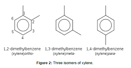
Xylenes are an aromatic compound with the general formula, C6H4(CH3)2 and an NFPA rating of two in health, three in flammability, and zero in reactivity [5]. There are three isomers of xylene, differing by the positions of the two methyl groups, as shown below in Figure 2.
While xylenes are considered physical irritants, and environmental pollutant, they are also heavily used in the manufacturing industry [5]. Xylenes are used in a variety of applications including raw materials for the production and synthesis of benzoic acid and terephthalic acid, which is a precursor to poly (ethylene terephthalate), or PET, a common plastic used as soda bottle containers [5]. Xylene is also commonly used as a solvent and is present in paints and adhesives; Rust-Oleum paint, and Klean-Strip being two well-known brands [6].
The catalytic disproportionation reaction of toluene to benzene and xylenes (three isomers: meta-xylene, para-xylene, and ortho-xylene) proceeds as: 2 Toluene → Benzene+Xylenes. Companies that use this reaction include both Mobil Corporation and UOP LLC [7]. Since 1976, the United States Patent Office has filed over 400 applications for patents regarding purification processes for para-xylene [8].
Most commercial uses of xylenes involve the mixture of the three isomers, but para-xylene (p-xylene) is the most desirable isomer [7]. Para-xylene is used in the production of polyester fibers, films, and other resins. Demand for p-xylene usually sees a steady demand growth of about 6-8% per year, so the need for separation and purification remains a high priority in the manufacturing industry [7].
Flowsheet analysis and pinch design
The disproportionation reaction of toluene to benzene and xylene isomers proceeds as: 2 Toluene → Benzene+Xylenes [9]. The mass and energy balances for the production process were obtained through ASPEN, along with the original reactor network. The information about the original process can be found in Appendix IA. Ten process streams were extracted from the flowsheet, as well as three reboilers and three condensers that corresponded to distillation columns, as can be seen in Table 1.
| Stream Designation | Stream Name | Supply Temperature (°C) | Target Temperature (°C) | Heat Capacity Flow Rate, CP (kW/°C) | Enthalpy Change, ∆H (kW) |
|---|---|---|---|---|---|
| 1 | M10--F11--F10 | 129 | 450 | 2.17 | 696.57 |
| 2 | R10--E21--E20 | 300 | 40 | 2.64 | 686.4 |
| 3 | Dil--E30 | 40 | 75 | 1.23 | 43.05 |
| 4 | T1V--E40 | 35.5 | 25 | 0.22 | 2.31 |
| 5 | T1L--T2F | 130 | 80 | 1.15 | 57.5 |
| 6 | T2V--E60 | 104.5 | 70 | 0.66 | 22.77 |
| 7 | SO--Benzene | 70 | 35 | 0.06 | 2.1 |
| 8 | T3L--P60--E120 | 249 | 25 | 0.12 | 26.88 |
| 9 | T3V--E90 | 80 | 183 | 3.2 | 329.6 |
| 10 | Rec,Out--Rec,In | 25 | 80 | 5.3 | 29.15 |
| 11 | QCOND,1 | 35.5 | 35.5 | -- | 35.7 |
| 12 | QCOND,2 | 104.5 | 104.5 | -- | 186.8 |
| 13 | QCOND,3 | 183.2 | 183.2 | -- | 2552.7 |
| 14 | QREB,1 | 130 | 130 | -- | 95 |
| 15 | QREB,2 | 150.4 | 150.4 | -- | 286.5 |
| 16 | QREB,3 | 249.4 | 249.4 | -- | 2832 |
Table 1: Toluene disproportionation flow data.
Once the data was extracted from the ASPEN data and flowsheet, a pinch analysis program in Excel was used to calculate the pinch temperature and minimum heating and cooling duties for the system with the integrated columns. The minimum temperature change for the streams was given as 10°C. The program was first run for a pilot scale process, and then for a full-scale process, which was ten times the size of the pilot plant. The process was assumed to be a linear scale-up; each of the values could be directly multiplied by ten. Table 2 shows the minimum heating and cooling duties, pinch temperature, and energy savings for the original process, the integrated pilot scale process, and the full-scale plant process. The energy savings from integration are considerably high, resulting in about 20% savings for heating, and 39% savings for cooling. The heat cascade, composite curves, and the network design can be found in Appendices IB-ID.
| QH,MIN (kW) | QC,MIN (kW) | TPINCH (°C) | Energy Savings: Heating (kW) | Energy Savings: Cooling (kW) | |
|---|---|---|---|---|---|
| Original Plant | 3953.2 | 3937.8 | -- | -- | -- |
| Integrated Pilot Scale Plant | 3160.12 | 2421.41 | 254.4 | 793.08 | 1516.39 |
| Full Scale Plant (10x Pilot Scale) | 31601.2 | 24214.1 | 254.4 | 7930.8 | 15163.9 |
Table 2: Heating duties, cooling duties, pinch temperature, and energy savings for the original plant and the fully integrated plants.
The heat released in the processes can also be used in order to raise steam. Using the properties of water (heat of vaporization of 2270 kJ/kg, and specific heat capacity of 4.184 kJ/kg∙K) and the composite curves, the amount of steam that could be raised from the process below the pinch was calculated. This amount of steam was determined to be 4.04 kg/hr. The data for steam generation can be found in Appendix ID3.
The heating and cooling duties for each of the plant designs could then be translated into an equivalent amount of coal, an equivalent energy coal cost, and the equivalent amount of carbon dioxide emissions per year, as shown in Table 3 below.
| Heat (kW∙hr) | Heat per Year (kW∙hr/yr) | Coal Equivalent (tons/yr) | Coal Costs (USD/yr) | CO2 Emissions (tons/yr) | |
|---|---|---|---|---|---|
| Original Plant | 3953.2 | 3.47E+07 | 1.51E+08 | 9.09E+09 | 2.77E+08 |
| Integrated Pilot Scale Plant | 3160.12 | 2.77E+07 | 1.21E+08 | 7.26E+09 | 2.22E+08 |
| Full Scale Plant (10x Pilot Scale) | 31601.2 | 2.77E+08 | 1.21E+09 | 7.26E+10 | 2.22E+09 |
Table 3: Cost and energy analysis for each plant schematic.
Table 4 puts Table 3 into perspective in terms of the full amount of savings realized from the new design of the process. The monetary CO2 savings were calculated by assuming that one carbon credit is equal to $10.00 per ton of CO2. By integrating the process, almost two and a half billion dollars can be saved just on the pilot process alone, and then 20 billion dollars on the full-scale plant. The parameters and conversions used in the cost analysis can be found in Appendix IE.
| Pilot Plant | Full Scale Plant | |
|---|---|---|
| Savings by Process Integration | 1.82E+09 | 1.82E+10 |
| CO2 Reduction per Year (tons) | 5.56E+07 | 5.56E+08 |
| CO2 Savings | 5.56E+08 | 5.56E+09 |
| Total Savings | 2.38E+09 | 2.38E+10 |
Table 4: Full cost savings from process integration.
Once the total savings associated with the new plant design were realized, a comparison of marginal costs and savings was made. The marginal dollar savings of energy and capital investment required to reduce energy consumption is given as a constant dollar amount regardless of the actual energy saved: $100 per megawatt (MW). The marginal capital costs associated with the new plant design is given by the expression: Capital Costs [$]=e5.1x, where x is the energy reduction in megawatts. The intersection of the marginal costs and the marginal savings gives the optimal energy savings to balance the costs. This optimal amount of energy savings is 0.903 MW, or 903 kW of energy. The plot for the costs and savings are shown below in Figure 3.
Using the information from the marginal cost and savings analysis, a new ΔTMIN value for the pinch analysis was derived in order for the process to be the most cost effective. A plot showing the savings and costs plotted against ΔTMIN can be found in Appendix IF. The intersection between the costs and savings represents the optimal temperature that should be run. This temperature was determined to be 87.5°C.
Reactor design
While there are many uses for both meta- and ortho-xylenes, as well as the mixture of all three, para-xylene is the most valuable of the three isomers. As a result, it is desirable to construct a reactor system for optimizing the concentration of p-xylene.
For the given temperature and catalyst conditions, the following chemical reactions occur:

Where mx denotes m-xylene, px denotes p-xylene, ox denotes o-xylene, and d represents a product that has little economic value. Each reaction has a rate constant associated with it, where k1=1.2 s-1, k2=1.5 s-1, and k3=1.1 L/mol∙s. The feed concentration of mx into the reactor is 0.5 mol/L, and the initial concentrations of px, ox, and d are 0 mol/L. The feed flow rate, F, is 1 L/s.
Five different reactor systems were modeled in order to determine the best system for optimizing px. Each of the systems was modeled using codes written in Mathematica, which can be found in Appendix IIC. The following rate equations [10] were used in modeling the kinetics, where the subscripts “mx”, “px”, “ox”, and “d” denote the species.

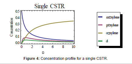
First, a single continuously stirred tank reactor (CSTR) was modeled using the governing equation for a CSTR:  where Ci,0 is the initial concentration of the species, Ci is the concentration of species i at a given time, dCi/dτ is the rate equation, and τ is the residence time [10-13]. Each of these equations was solved for each of the species. The full set of equations can be found in Appendix IIA. The resulting concentration profile for the CSTR is shown in Figure 4 below, where the peak concentration of px reaches 0.084 mol/L at a residence time of 0.738 seconds.
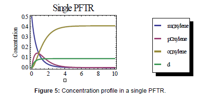
Next, a plug flow tubular reactor (PFTR) was modeled using the rate equations as given above and integrating each of the differentials to obtain a concentration profile. The resulting graph of the concentrations as a function of time is shown below.
In the model using the PFTR, the peak concentration of px occurs at a residence time of 0.671 seconds and is 0.143 mol/L, almost double the peak concentration of px in the CSTR. So, the PFTR is the most optimal compared to the CSTR system.
Other systems modeled include two CSTRs in series, a PFTR with a 50% recycle stream, and a PFTR and CSTR in series. Each of the graphs of the concentration profiles can be found in Appendix IIB. Table 5 below indicates the resulting values of the concentration of px, the residence time that the concentrations occur at (the optimal residence time), and the percent yield of px (where the yield is calculated as
Table 6 shows that both the single PFTR and the PFTR with the same peak concentration of px. But, the PFTR with the recycle stream takes longer to reach that concentration. Since the optimal volume of the reactor system is calculated as VOPTIMAL= ƮOPTIMAL. F, where F is the feed flow rate (which is 1 L/s), the optimal volume would be the small volume in order to save on capital costs of the reactor. So, the single PFTR would be more optimal to use than the PFTR with the recycle stream. As can be seen from the table, each of the other systems reach a peak concentration of px that is less than that of the single PFTR. Furthermore, the yield of the px in the single PFTR system is higher than in the other reactor systems, and agrees with the literature value of 25% [9]. So, the single PFTR would be the best reactor choice for optimizing the concentration of px.
| System | τOPTIMAL (s) | Cp-xylene (mol/L) | Yield (%) |
|---|---|---|---|
| 1 CSTR | 0.738 | 0.084 | 16.80% |
| 1 PFTR | 0.671 | 0.143 | 28.50% |
| 2 CSTRs in Series | 0.238 | 0.097 | 19.40% |
| PFTR with 50% Recycle | 1.007 | 0.143 | 28.50% |
| PFTR then CSTR in Series | 0.25 | 0.113 | 22.60% |
Table 5: Optimal resident times, concentrations of p-xylene and percent yield for each modeled reactor system.
| Single PFTR | |
|---|---|
| τOPTIMAL (s) | 0.671 |
| F (L/s) | 1 |
| VOPTIMAL (L) | 0.671 |
| Cp-xylene (mol/L) | 0.143 |
| Cm-xylene (mol/L) | 0.178 |
| Co-xylene (mol/L) | 0.104 |
| Cd (mol/L) | 0.075 |
Table 6: Resulting concentrations of xylene isomers and product at the optimal residence time for a single PFTR.
As a result, the optimal residence time for the single PFTR is 0.671 seconds. The following table shows the concentrations of the other species, and the operating conditions for this system.
While this PFTR reactor optimizes the yield of px to the literature value of 25%, new processes have been developed in recent years, with the most notable being the PX-PlusTM process from UOP LLC [9], where the toluene → benzene+xylenes reaction proceeds with paraxylene selectivity, giving a yield of 90% of px [9].
Heat exchanger dynamics
The dynamic profile of a single pass shell and tube, counter current heat exchanger can be modeled using the one dimension heat exchanger equation,  where T is the temperature of the stream, TS is the temperature of the counter current stream in the shell (for this design, the counter current stream is steam), t is the time in seconds, and z is the length in meters along the exchanger. Other variables in the equation include the velocity of the stream, v, the overall heat transfer coefficient, U, the heat transfer area per unit length, S, the specific heat capacity of the stream, Cp, the density of the fluid, ρ, and the area of the heat exchanger, A.
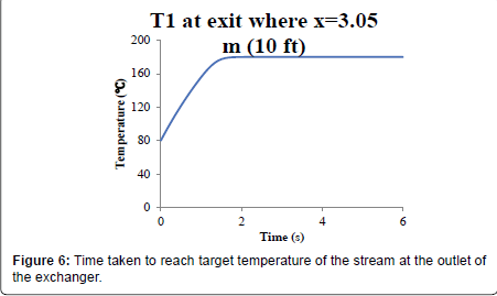
Numerical solution: The numerical (finite element) dynamic solution of the stream provided a feasible estimation of the steam temperature needed to increase the stream temperature from 80°C at the inlet to 180°C at the outlet for a 10-foot exchanger with a stream velocity of 1.5 m/s. The input data and tables can be found in Appendix IIIA. Figure 5 shows the stream profile with the temperature of the steam, Ts, of 322.5°C. The temperature of the stream reaches the target exit temperature of 180°C after 1.6 seconds. Figure 6 shows the temperature profile of the stream along the exchanger after it reaches steady state.
Progression of the temperature increase in the stream was also modeled and can be seen in Figures 7 and 8 in increments of time until the target temperature and steady state conditions were reached.
Analytical solution: The solution to the heat exchanger equation,  can also be calculated in an analytical way. The equation can be classified as a linear partial differential equation of temperature. The equation is not solvable by separation of variables. Instead, the equation must be solved by the method of characteristics [11].
The method of characteristics is used for equations of the form: The solution for the function is calculated hrough the use of a system of auxiliary system of equations:
  , with the solution to the equation,
 being calculated as: bxay= c. The second equation is then
  The solution to this second equation follows the form:
  for an equation where f(x,y) is a constant and the coefficients, a and b are constants So, the heat exchanger equation can be rearranged to be:
 where
where As a result, the temperature profile for the system becomes:
References
- Coal Receipts at Commercial and Institutional Users by Census Division and State (2009) Energy Information Administration.
- Cost of Coal Delivered to Electric Generating Plants (2009) Energy Information Administration: Washington, DC, USA.
- Carbon Dioxide Emissions by Sector and Source (2009) aeotab_18.xls. Energy Information Administration: Washington DC, USA.
- Occupational Safety and Health Guideline for Xylene (2009) Accessed 18 November 2009.
- Klean-Strip Citri-Strip House Brite Armor (2004) WMBÂ Company. Memphis.
- Rust-Oleum American Accents Gloss Aerosol (2006) Rust-Oleum Corporation. Vernon Hills.
- Abichandani JSB, Brown SH, Cimini RJ, Kwok S, Johnson ID, et al. (1999) Para-Xylene Production process. WO/2000/010944.
- Wantanachaisaeng PO (2007) The Aromatics (Thailand) Public Co. Ltd. Capturing Opportunities for Para-xylene Production. In the Aromatics (Thailand) Public Co. Ltd., UOP: Des Plains.
- Para-xylene and Purification (2009) In United States Patent Collection, United States Patent Office.
- Schmidt LD (2005) The Engineering of Chemical Reactions. 2nd edn. Oxford University Press, New York.
- Kythe PK, Schaferkotter MR (1997) Partial Differential Equations and Mathematica. CRC Press, Boca Raton, USA.
Citation: Mongelli GF, Dougherty L, Wang S (2018) Chemical Process Design for Manufacture of Xylene Isomers. Ind Chem 4: 125 DOI: 10.4172/2469-9764.1000125
Copyright: © 2018 Mongelli GF, et al. This is an open-access article distributed under the terms of the Creative Commons Attribution License, which permits unrestricted use, distribution, and reproduction in any medium, provided the original author and source are credited.
Share This Article
Recommended Journals
Open Access Journals
Article Tools
Article Usage
- Total views: 8633
- [From(publication date): 0-2018 - Apr 03, 2025]
- Breakdown by view type
- HTML page views: 7040
- PDF downloads: 1593


