Cartography of Extreme Rainfall and Their Relationship with Topography in the French Alps
Received: 21-Mar-2018 / Accepted Date: 10-Jun-2018 / Published Date: 15-Jun-2018 DOI: 10.4172/2157-7617.1000477
Abstract
The extreme rains of court duration are the principal cause of brutal and catastrophic flood that can be produced on a nombre of smal bassin on the french Alps. This study consists on a cartography of extraim values of pluviometric parametres, as a Gradex, rains with a period of 10 years, 100 years and 1000 years, for six steps of time (1 h, 2 h, 3 h, 6 h, 12 h, 24 h); and Montana parameter on the french Alps where the orographic effect is big and the estimation of reliables values on unmonitored site using data of environmental stations need the introduction of morphometric informations. The areA study covers a surface of 250 km × 450 km and dispose of 65 oluviometrics stations of average durations between 30 and 35 years. This study has been done on two steps, first we have done a presentation of a region by a relief and a climate, second, we have displayed pluviometrics systems using ACP method. The idea based on AURELHY method (Analysing Using Relief for HYdrometeology) that consists to intervene the local topography by a lineair regression and analysing by kriging the residu of the regression has been used for this cartography.
Keywords: Extreme rains; Hydrology; Morphometry; Linear regression
Introduction
We have a network of rainfall stations distributed unevenly over a field of study. On each of the stations, we have estimated some parameters related to the rain. Each of the estimated parameters is related to a variable distributed at the station, according to a given probability law, of central value equal to the estimated parameter. The error made in estimating a parameter will be inversely proportional to the square root of the sample size. It will be a sampling error. it will not be the only one. Indeed, the identification of each law of probability is made of sample of which each element is measured with a certain error. The goal is to be able to connect, according to a linear model, the parameters of the rain to other parameters which concern the relief.
The relief parameters, which would affect the rain are they varying for each station. In the framework of the model, they will be assumed without error (this hypothesis largely simplifies the model).
Implementation
The idea is to map the fields of precipitation characteristics taking into account as much information as possible. The first information is of course the point estimates of extreme rainfall for different time steps. We want to know the number of parameters that can characterize the site and look for other parameters that can affect the distribution of precipitation: the altitude of the precipitation station, the longitude measured by Lambert x, the latitude measured by y Lambert, the average altitude calculated on a few M.N.T fixed nodes closest to the station [1-5].
Precipitation can therefore be considered as a function of three components:
R(x)=f(Rsit e(x), Rsituation (x), Rrégion (x))
The work consisted to identify what is the site and varies too quickly to be mapped from the only rainfall data point.
The only features of the region are of course the xj and the yj.
Compos antes Principals Relief
The main components of the relief cp1, ... cp10, which are only calculated at the rainfall stations for a M.N.T step is 2 km
From a numerical model of ground whose step = 2 km applied on our field which makes 250 km/450km is a matrix of altitudes of 225 lines and 125 columns, one seeks to calculate the principal components of the relief while taking the radius of influences of the assumed relief over the rainfall equal to 4 km, which equals a radius equal to 4 meshes and therefore the landscape surrounding the point "o" is a matrix (9 × 9) mean altitudes and this site will be characterized by altitudes at the level of the 81 nodes of the mesh and thus by 81 values. 25389 sites in the French Alps area can be identified from the DTM (excluding the 4 most eastern columns, the 4 westernmost columns, the 4 southernmost lines, and the 4 most southerly lines). North).
The application of ACP to the z matrix (25389.89) shows the following results:
The first 8 main components account for more than 90% of the field variance (85% for the top 5)
From the figure log (λk) = f (k) we see that only 6 components are sufficient to summarize the relief.
Each Eigenvector aik appears as a basic landscape and is clearly clear.
αi1: Cashing effect (35% variance explained)
αi2: Presence of a north-west/southeast slope (22% explained variance)
αi3: Presence of a southwesterly/northeasterly slope (18% variance explained)
αi4: Collar effect (6% of explained variance)
αi5: Collar effect (4% of variance explained)
αi6: Unclear effect
αi7: Unclear effect
αi8: Unclear effect
we reported the eight fields of αi1, αi2, αi3, αi4, αi5, αi6, αi7, αi8 as illustrated by the first eight major components of relief. The site environment is a linear combination of these eight basic "landscapes". These basic landscapes are drawn on a surface grid (8 × 8) km and not equal to 2 km and whose basic data are the relative altitudes calculated at the 24 nodes of the grid with respect to the central node.
Basic Landscape # 1 illustrates the existence of a depression or summit around the central point. Landscape # 2 expresses a downward slope to the northwest or a downward slope to the South East. The third landscape shows a slope either descending northeast or southeast direction northwest, the fifth landscape also shows a neck effect, but direction is east-west or north-south. Basic Landscapes No. 6, 7, 8 reveal finer spatial structures not easy to interpret.
Distance from the Fireplace of Ellipse des Alpes
After a long reflection on the problem of the relationship between the characteristics of the extreme rainfall and the relief in this region, we thought that it could be the look of the alpine chain which draws like elliptical arcs continuing from the Mediterranean to the west. As far as the Jura in the east, may be of importance, and we may say that the characteristics of extreme rain are related to the distance separating a given station from the two foci of an ellipse having the same aspect as the chain, we then traced by hand an elliptical arc having the shape of the chain, from a dozen points taken on this arc, we sought these two foci which are f1 (x=950 km, y=240 km) f2(x=1025, y=450 km).
The new variable to introduce in the regression riding is the distance of each station to the two f1 and f2 foci and that we will note "dist".
Regression Pluviometrie-Morphometrie

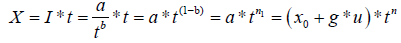
I: Intensity of the rain
A: Rain for a return period and a given duration
Finally, we can write

x0: position parameter
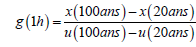
g: Grade
u: Reduced variable of Gumbel
n: Montana setting;
t: No time
T: The return period
Knowing the map x0, the grade and the Montana parameter we will be able to determine the value of the rain for any time step and any return period and at any place of the field, so we decided to draw the three maps (x0(x,y), g(x,y) et n(x,y)), at the beginning we took the step of the time of 1h and the grade was calculated for the return periods of 20 years and 100 years.
For the Montana parameter we took a mean value between the one calculated for T = 20 years and T = 100 years that we called nmoy
nmoy = ( n(20 ans)+n(100ans))/2
n(20ans): Montana parameter calculated on the rain of 20 years
n(100ans): Montana parameter calculated on the 100-year-old rain
And x0 will be the rain for T=20 years and t = 1h and that we note x (1h, 20 years)
We looked for the regression between x (1h, 20years), g (1h), and nmoyand the different explanatory variables, namely the main components of the relief, the regional parameters, the altimetric parameters and the distance from the focal points of the ellipse, we find as results:
x(1 h,20 ans)=8.31 × 10⁻² X -3.05 × 10⁻² Y+0.112629 dist-77.29678 R=80.68%
g(1 h)=1.51 × 10⁻² X - 8.21 × 10⁻³ Y+2.32 × 10⁻² dist - 13.19608 R=72.95%
nmoy= 1016 × 10-4 Z+0.29048 R=59.34%
We note that for the rain x (1 h, 20 years) the more we sink into the chain (the distance to the homes increases) the more it rains, the altitude does not intervene, and this is explained by the fact that the rain is stormy type, that is to say that the convective motions of humid air masses causing thunderstorms are, indeed, in fact, not a priori not related to the study of the fluviometric position. For the time grade we also note that the more we sink into the chain plus the grade is high and the term altitude does not intervene. On the other hand, the Montana parameter is explained using a single variable, which is the altitude, and which has a positive sign meaning that this parameter is strong on the bumps and weak in the hollows.
After having drawn the maps of the hourly rain of 20 years and that of the grade we see that they have a very smooth shape and that is a thing planned; we preferred to work on other no time where the altitude could play a role and it was thought that it would be better to consider the rain and the grade for the step of 24 hours (Tables 1-6).
| Variable | Equation | R2 % |
|---|---|---|
| x(1 h, 20 ans) | 8.31 × 10⁻² X -3.05 × 10⁻² Y+0.112629 dist-77.29678 | 65.09 |
| g(1 h) | 1.51 × 10⁻² X - 8.21 × 10⁻³ Y+2.32 × 10⁻² dist - 13.19608 | 53.22 |
| x(24 h, 20 ans | 0.271666 X -7.62 × 10⁻² Y+2.28 × 10⁻² Z +0.32137 dist-248.3298 | 38.85 |
| g(24 h) | 0.5636 × 10⁻¹ X – 0.2455 × 10⁻¹ Y+4.0862 × 10⁻³ dist – 50.49 | 38.20 |
| nmoy | 1016 × 10-4 Z+0.29048 | 35.27 |
Table 1: Regression of rainfall variables.
| Variable | Coefficient of regression | Partial correlation coefficient |
|---|---|---|
| X | 8.31 × 10⁻² | 0.454525 |
| Y | -3.05 × 10⁻² | -0.5055519 |
| dist | 0.12629 | 0.7542605 |
Table 2: Hourly rainfall of 20 years.
| Variable | Coefficient of regression | Partial correlation coefficient |
|---|---|---|
| X | 1.51 × 10⁻² | 0.3346648 |
| Y | -8.21 × 10⁻³ | -0.5175238 |
| dist | 2032 × 10-2 | 0.6293096 |
Table 3: Hourly gradex.
| Variable | Coefficient of regression | Partial correlation coefficient |
|---|---|---|
| X | 0.271666 | 0.4545525 |
| Y | -7.62 × 10⁻² | -0.5055519 |
| Z | 2.28 × 10⁻² | 0.3657714 |
| dist | 0.321374 | 0.5089973 |
Table 4: Daily rain of 20 years.
| Variable | Coefficient of regression | Partial correlation coefficient |
|---|---|---|
| X | 5.636 × 10⁻² | 0.29903 |
| Y | -2.455 × 10⁻² | -0.39540 |
| Z | 4.0862 × 10⁻³ | 0.24804 |
| dist | 6.557 × 10⁻² | 0.42874 |
Table 5: Daily gradex.
| Variable | Coefficient of regression | Partial correlation coefficient |
|---|---|---|
| Z | 1.16 × 10⁻⁴ | 0593899 |
Table 6: Montana.
We find the following regression equation:
x(24 h,20 ans)=0.271666 X -7.62 × 10⁻² Y+2.28 × 10⁻² Z +0.32137 dist-248.3298 R=62.33%
g(24 h)=0.5636 × 10⁻¹ X – 0.2455 × 10⁻¹ Y+4.0862 × 10⁻³ dist – 50.49 R=61.81%
Interpretation
The latitude, longitude and distance to home variables best explainthe 20-year rainfall with a multiple correlation coefficient of 0.807. if we look at the partial correlation coefficients, we find that the distance variable has the greatest coefficient of the order of 0754, while that of the other two explanatory variables latitude and longitude do not exceed the value of 0.5 in absolute value (respectively -0.506 and 0454), we conclude that it rains more on the outer slopes of the Alps directly exposed to humid air masses. The variable altitude does not intervene that it is the altitude of the post or the surrounding altitudes what is explained by the fact that this rain is of the storm type provoked by the encasement of the valleys favouring the descent along the high reliefs.
For the time grade the regression equation allows us to reach a value of correlation coefficient of the order of 0.7295 but which remains less than that of the twenty-hour rain hourly. They are the same explanatory variables that appear in the same order and with the same sign: the longitude first with a positive sign, then the latitude with a negative sign and the distance in third position with a positive sign. The latter has the highest partial correlation coefficient (0.629) which is about twice that of longitude (0.3346), and much larger than latitude (-0.5175), meaning that the effect of distance Home is the most important and so the further down the chain in the direction of the west the higher the grade is.
For the 20-year-old rain, in addition to the usual variables a variable that appears which is the altitude, with a positive sign, it returns in third position after the longitude and the latitude. All variables have positive sign regression coefficients except latitude.
The partial correlation coefficient of the distance variable decreases (0.5) compared to that of the hourly rain, which is recovered by the effect of the altitude whose partial correlation coefficient reaches the value of 0.3658. the latitude and longitude variables retain their partial correlation coefficient value. We conclude that the more we sink west in the chain plus this rainfall parameter is plentiful, especially on the bumps in the hollows.
For the daily grade we find the appearance of the altitude variable to be compared with the hourly grade, the multiple correlation coefficient has decreased (0.62) the partial correlation coefficients of the different variables (longitude, latitude and distance) have decreased, as for the rain.
At 24 h, the appearance of the altitude effect decreased the effects of the other variables, although the effect of distance remains at the top with a partial correlation coefficient of 0.4287. the daily grade increases moving further east to west, especially as the altitude is high.
The only explanatory variable of this parameter is the altitude with a positive sign. The coefficient of multiple correlation is of the order of 0.5934 meaning that this parameter is strong on the bumps and weak in the hollows [6-10].
Discussion and Conclusion
The principal components analysis shows that the space of the 19 rainfall parameters can be reduced to an equivalent space of dimension 2 and practically some is the dimension of the space of the parameters it is always reduced to a space in two dimensions provided that there is the Montana parameter. The space of the stations of dimension 50 is reduced to an equivalent space of dimension 5. Therefore, the rainfall information observed on the 50 stations is equivalent to 2 rainfall parameters measured on 5 average stations each of which represents a class.
The relief analysis shows that each landscape in the Alpine region is a combination of the six basic landscapes obtained. The use of these landscapes in the rainfall-morphometric regression did not give spectacular results surely because the mesh of M.N.T is not sufficiently fine. it is the latitude, longitude, altitude of the rainfall post and the distance from the households that play the greatest role in this regression.
References
- Benichou P, Lebreton O (1986) Taking into account the topography for the mapping of statistical rainfall fields. Meteorology 2: 1.
- Blanchet G (1993) Variability of annual rainfall in the Rhône-Alpes region: Cartographic presentation. Lyon Geography Review 68: 2-3
- Braud I (1990) Methodological study of principal component analysis of two-dimensional processes. Effect of numerical approximations and sampling and use for the simulation of random fields: Application to the treatment of monthly sea surface temperatures on the intertropical Atlantic. 16: 32-38.
- Creutin D (1979) Optimum interpolation method of hydro-meteorological fields comparison and application to a series of rainy episodes Cevennes. Thesis of doctor-engineer. INP Grenoble.
- Desurosne I (1992) Gradient of rainfall intensities in relief zones: Experiments and first data modeling of a Rhône-alpine network, the TPG. Thesis of the University Louis Pasteur. Strasbourg.
- Laborde JP (1984) Data analysis and automatic mapping in hydrology lorraine hydrology element PhD thesis. INPL Nancy 2: 1.
- Laborde JP (1982) Automatic mapping of rainfall characteristics: Taking into account pluviometry-morphometric relationships.
- Obled CH (1979) Contribution to the analysis of data in hydrology: The prediction of accidental phenomena and the analysis of spatial fields" Thesis of space fields "Thesis of State. USMGINP Grenoble.
- Slimani M (1985) Study of rare frequency rains at short time steps in the Cévennes-Vivarais region: Estimation, relationship with relief and synthetic mapping. Thesis Doctor-Engineer, I.N.P Grenoble.
- Tourasse P (1981) Spatial and temporal analyzes of precipitation and operational use in a flood forecasting system. Application to the Cevennes regions, Thesis Doctor-Engineer. USMG-INP Grenoble.
Citation: Samia S, Bois P (2018) Cartography of Extreme Rainfall and Their Relationship with Topography in the French Alps . J Earth Sci Clim Change 9: 477. DOI: 10.4172/2157-7617.1000477
Copyright: © 2018 Samia S, et al. This is an open-access article distributed under the terms of the Creative Commons Attribution License, which permits unrestricted use, distribution, and reproduction in any medium, provided the original author and source are credited.
Select your language of interest to view the total content in your interested language
Share This Article
Recommended Journals
Open Access Journals
Article Tools
Article Usage
- Total views: 3929
- [From(publication date): 0-2018 - Nov 04, 2025]
- Breakdown by view type
- HTML page views: 3056
- PDF downloads: 873