Breast Cancer Prediction by Logistic Regression with CUDA Parallel Programming Support

Continuous advancements in the field of statistical model research as well as the improvement of informatics technologies have opened new scenarios, including the application of different methodologies for analysing data, extracting knowledge through models and predicting some kind of stuffs. In the present article a model based on the analysis of some digital data, triggered by real data source, was developed to assess if a patient has a malignant or benignant breast cancer [1]. The approach is non-invasive, and is based on a model consisting in a learning algorithm approach. With the support of new technologies and storage techniques, large amount of cancer data are collected and can become available for the whole community. Such a kind of data was used to develop and test the model proposed in the present work.s

Large number of risk prediction models have been developed that evaluate different types of risk factors for breast cancer tumor and not only. The most famous models are those of Gail, Claus, Tyrer-Cuzick and the Jonker [2]. These predictions models are also called prognostic models. The basis of the prognostic models are the type of risk factors evaluated for getting the prognosis such as family history, life habits, etc. [3,4].

Logistic regression is used also to predict whether a patient has a given disease such as diabetes, coronary heart disease, breast cancer based on observed characteristics of the patients such as age, sex, body mass indexes and blood tests or through digitalized data [5,6]. The mathematical model could be used in demographic challenges such as the prediction of the choose of an American voter [7] or in engineering for predicting the likelihood of failure of a specific process [8,9].

In this study the logistic regression was used for creating a model upon the breast cancer disease. The system we have developed consists in the estimation of unknown dependencies in a system from a given dataset to create a useful and general model to analyse new incoming data. Furthermore, the system is developed to be used on NVIDIA hardware to take advantages of Parallel Programming technique through Theano framework.

For obtaining a reasonable model, we did use a real dataset delivered by Wisconsin Diagnostic Breast Cancer database where it is filled by real data from patients. The database has 569 instances and each one correspond to a patient. This type of data are anonymized because of they are sensitive and private data.

Data set: Technical information

In Figure 1, technical information of the input data set is shown. Features are computed from a digitized image of a fine needle aspirate (FNA) of a breast mass [10]. They describe characteristics of the cell nuclei present in the image. Separating plane described above was obtained using Multisurface Method-Tree (MSM-T), a classification method which uses linear programming to construct a decision tree. Relevant features were selected using an exhaustive search in the space of 1-4 features and 1-3 separating planes. The actual linear program used to obtain the separating plane in the 3-dimensional space is reported in literature [11].

Figure 1: Technical information about used data set

The numbers of instances represent the number of patients and for each patient 32 digit-attributes are available. The first value represents the patient ID, the second one is the diagnosis value (M or B) of the patient and the remaining values are the real-valued input features taken by FNA. The values for the diagnosis value can be:

M = Malignant tumour; B = Benignant tumour;

The right interpretation of the data set is fundamental to create a good model and a good simulation close to reality over logistic regression. In particular it is essential to highlight the dependent variable y (belonging class) and the independent variables x1….xn. The diagnostic value is in the model the dependent variable y and it has a value range of [0,1] because it assumes value M or B, while the real-valued input could be the independent variables xn representing the qualitative variables.

NVIDIA CUDA

Parallel Programming: The authors decided to create the model upon the NVIDIA Hardware to take advantages of parallel computations. It enables dramatic increases in computing performance by harnessing the power of the graphics processing unit (GPU). CUDA is built around a scalable array of multithreaded Streaming Multiprocessor (SMs) [12]. So, the kernel executes a grid of threads blocks at the same time. This model can be called as SIMT (Single Instruction Multiple Data) and it means that a single instruction is performed over multiple data together. The choice to use this type of technologies was done because of It could be possible to reduce the amount of execution time even if the input data-set is not huge. Furthermore, the authors want to take care about the future development and a consequent increment of input data.

Pearson correlation coefficient

Before the creation of the model we analysed deeply the input data to understand if there are some types of correlation between them [13]. We used the Pearson correlation coefficient [14], box plot and parallel plot. In particular, Pearson coefficient measures how well data are related. Definitely, it cannot able to measure the relation between dependent and independent data. In Figure 2 we find a graphical representation of the Pearson Correlation Coefficient of input data set.

Figure 2: Pearson Correlation Coefficient of the input dataset

Figure 2 highlights a scattered correlation among the data. It means that the variables are linear independent and so we couldn’t apply reduction procedures (e.g. Principal Component Analysis).

Furthermore, due to the independence of the data we have chosen to use logistic regression. We deep analyze the logistic regression approach in section 3, “Algorithm”.

Box plot chart: Figure 3 is a box plot representation, in which we can notify that only in 3 clinical variables there are some outliers belonging to the malignant class, but the same patients do not exhibit other anomalies in the order values and so is not possible to push out them from our dataset.

Figure 3: Box plot graph of the input dataset

Parallel plot chart: Figure 4 represents the parallel-plot [15]. It can be used to verify if there is a strong separation between the clinical variables that belong to the two classes but in that case it confirms the result has been shown in the box-plot [16], there is not a strong separation between the classes.

Figure 4: Parallel plot graph of the input dataset

Algorithm

Logistic regression is a probabilistic, linear classifier. It is parameterized by a weight matrix W and a bias vector b. Classification is done by projecting an input vector onto a set of hyperplanes, each of which corresponds to a class. The distance from the input to a hyperplane reflects the probability that the input is a member of the corresponding class.

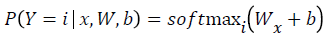
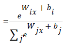
Mathematically, the probability that an input vector X is a member of a class i, a value of a stochastic variable Y, can be written as:

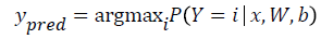
The model’s prediction Ypred is the class whose probability is maximal, specifically:

Since the parameters of the model must maintain a persistent state throughout training, they are allocated shared variables for W, b. This declares them both as being symbolic Theano variables, but also initializes their contents. The dot and softmax operators are then used to compute the vector. The result p y given x is a symbolic variable of vector-type.

To get the actual model prediction, we used the T. argmax operator, which returned the index at which p y given x is maximal (i.e. the class with maximum probability).

The right interpretation of the dataset is fundamental to create a good model and a good simulation as close to reality over logistic regression. In particular, it is important to highlight the dependent variable Y and the independent variables x1….xn. The diagnosis value could be in the model the dependent variable y and it has a value range of [0,1] because it assumes value M (Malignament) or B (Benignant) while the real-valued input could be the independent variables xn representing the qualitative variables.

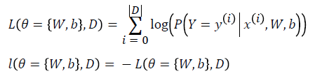
Learning optimal model parameters involves minimizing a loss function. In the case of multi-class logistic regression, it is very common to use the negative log-likelihood as the loss. This is equivalent to maximizing the likelihood of the data set under the model parameterized by Ɵ.

Let us first start by defining the likelihood and loss: L

Logistic regression is split in two phases. First of all there is the training phase wherein one sample is taken from the input dataset to learn the best value of the parameters W and b. Finally, there is the test phase where model previously trained is tested to see the response. Of course, the “learning process”, belonging to the training phase, is the most important part.

Implementations

In this section we have shown system implementation of system and the results obtained. Every version of the software is computed with CUDA Nvidia technology. The two versions differ due to the number of instances of the input dataset used for the training phase.

In particular in 1.0 version all the instances of the dataset are used to training the algorithm. Values of W and bias vector b are randomly chosen at the computation beginning. The result of each instance called y logistic is compared with the real diagnosis y real value belonging to input dataset to analyse the correct prediction of the values. The results in percentage are shown in Figure 5.

Figure 5: Simulation results algorithm version 1.

The pink bin represents the correct prediction of the algorithm. So, from the legend:

1. 482 right values. The value represents that on 569 patients the number of right predictions of the model is equal to 482 (85% right values).

2. 87 wrong values.

The last version model doesn’t use all the data set instances to perform the test phase. In version 2.0 training phase is composed by 85% of the instances of the whole input data set and it is used to “train” the algorithm (W and b values). The rest of the instances (15%) are performed to compute the test phase. For the training phase the percentage results are shown in Figures 6 and 7.

Figure 6: Training phase: simulation results algorithm version 2.

Figure 7: Test phase: simulation results algorithm version 2.

There is a main classification related to the machine learning algorithms: supervised and unsupervised methods. Supervised methods take a known set of input data, known responses to the data (output), and train a model to generate reasonable predictions for the response to new data. Unsupervised approaches, instead, draw inferences from input datasets without labelled responses. Logistic regression and artificial neural network belong to unsupervised learning approaches and they are the most widely used methods [17] in biomedicine and social science. Other methods can be found such as k-nearest neighbours, decision trees and support vector machines. From the Medline database it was possible to find 28,500 articles for logistic regression, 8500 for neural networks, 1300 for k-nearest neighbours, 1100 for decision trees, and 100 for support vector machines.

For example the TRISS which is “Trauma and Injury Severity Score”, is used to predict mortality in injured patients, was originally developed using logistic regression [11,18]. Another approach has proposed a parametric bootstrap model for a more accurate estimation of the prediction error specifically in microarray data trough logistic regression. The proposed method provides guidance about the selection of the number of genes and the optimal shrinkage for the penalized logistic regression. Their use in analyzing Golub's leukemia data and the cervical cancer data leads to highly accurate prediction models with a substantial reduction of the prediction errors.

The comparison of the two different versions indicates that for specific input data set the best performance are obtained with the version 2.0. In 1.0 version it is difficult to code the values for the coefficients of the model W and b, while in the second approach is a smart algorithm that can optimize the W value. Of course this is not a gold standard, but is an important to test the results using some different patient's cohorts and train again the model.

The results obtained from the simulation are important to improve the model and to work with it in future. The type of prognostic value obtained from logistic regression model could be used for a smart exams waiting list. If a patient has a y-logistic belonging to malignant breast cancer, she should have the priority for further analysis such as echography, bloods test, etc.

Thanks to “Bache K and Lichman M (2013). UCI Machine Learning Repository [http://archive.ics.uci.edu/ml]. Irvine, CA: University of California, School of Information and Computer Science” for the real data set of breast cancer tumour available.

References

- Ely S, Vioral AN (2007) Breast Cancer Overview. Plastic Surgical Nursing 27:128-133.
- Jacobi CE, de Bock GH, Siegerink B, van Asperen CJ (2009) Differences and similarities in breast cancer risk assessment models in clinical practice: which model to choose? Breast Cancer Res Treat 115: 381-390.
- Williams C, Brunskill S, Altman D, Briggs A, Campbell H, et al. (2006) Cost-effectiveness of using prognostic information to select women with breast cancer for adjuvant systemic therapy. Health Technol Assess 10: 1-204.
- Altman DG (2009) Prognostic models: a methodological framework and review of models for breast cancer. Cancer Invest 27: 235-243.
- Truett J, Cornfield J, Kannel W (1967) A multivariate analysis of the risk of coronary heart disease in Framingham. J Chronic Dis 20: 511-524.
- Freedman DA (2009) Statistical Models: Theory and Practice. Cambridge University Press 128.
- Harrell, Frank E (2001) Regression Modeling Strategies. Springer-Verlag.
- Strano M, Colosimo BM (2006) Logistic regression analysis for experimental determination of forming limit diagrams. International Journal of Machine Tools and Manufacture.
- Palei SK, Das SK (2009) Logistic regression model for prediction of roof fall risks in board and pillar workings in coal mines: An approach. Safety Science 47-88.
- Lever JV, Trott PA, Webb AJ (1985) Fine needle aspiration cytology. J ClinPathol 38: 1-11.
- Boyd CR, Tolson MA, Copes WS (1987) Evaluating trauma care: the TRISS method. Trauma Score and the Injury Severity Score. J Trauma 27: 370-378.
- Nickolls J, Buck I, Garland M, Skadron k (2008) "Scalable Parallel Programming with CUDA," ACM Queue 6: 40-53.
- Fayyad UM, Shapiro GP, Smyth P, Uthurusamy R (1996) Advances in Knowledge Discovery and Data Mining.
- Benesty J, Chen J, Huang Y, Cohen I (2009) Pearson Correlation Coefficient 2: 1-4.
- Robert ME (2003) The parallel coordinate plot in action: design and use for geographic visualization. Computational Statistics & Data Analysis 43: 605- 619.
- Williamson DF, Parker RA, Kendrick JS (1989) The Box Plot: A Simple Visual Method to Interpret Data. Ann Intern Med 110: 916- 921.
- Dreiseitla S, Machado LO (2002) Logistic Regression and Artificial neural network classifications models: a methodology review. Journal of Biomedical Informatics 35: 352-359.
- Liao JG, Chin KV (2007) Logistic regression for disease classification using microarray data: model selection in a large p and small n case. Bioinformatics 23: 1945-1951.
Citation: Peretti A, Amenta F (2016) Breast Cancer Prediction by Logistic Regression with CUDA Parallel Programming Support. Breast Can Curr Res 1: 111. DOI: 10.4172/2572-4118.1000111
Copyright: ©2016 Peretti A, et al. This is an open-access article distributed under the terms of the Creative Commons Attribution License, which permits unrestricted use, distribution, and reproduction in any medium, provided the original author and source are credited.
Share This Article
Recommended Journals
Open Access Journals
Article Tools
Article Usage
- Total views: 15157
- [From(publication date): 9-2016 - Jan 05, 2025]
- Breakdown by view type
- HTML page views: 14316
- PDF downloads: 841