Assessment of Levee Erosion Using Image Processing and Contextual Cueing
Received: 13-Jul-2018 / Accepted Date: 23-Jul-2018 / Published Date: 30-Jul-2018
Abstract
Soil erosion is one of the most severe land degradation problems afflicting many parts of the world where topography of the land is relatively steep. Due to inaccessibility to steep terrain, such as slopes in levees and forested mountains, advanced data processing techniques can be used to identify and assess high risk erosion zones. Unlike existing methods that require human observations, which can be expensive and error-prone, the proposed approach uses a fully automated algorithm to indicate when an area is at risk of erosion; this is accomplished by processing Landsat and aerial images taken using drones. In this paper the image processing algorithm is presented, which can be used to identify the scene of an image by classifying it in one of six categories: levee, mountain, forest, degraded forest, cropland, grassland or orchard. This paper focuses on automatic scene detection using global features with local representations to show the gradient structure of an image. The output of this work counts as a contextual cueing and can be used in erosion assessment, which can be used to predict erosion risks in levees. We also discuss the environmental implications of deferred erosion control in levees.
Keywords: Contextual cueing; Machine learning; Soil erosion; Erosion control; Image processing
Introduction
Soil erosion is defined as a displacement of solid particles originating from soil, rock, and other sediments. Soil is naturally removed by the effect of water, wind, ice, and/or by downward (or down-slope) movement caused by gravity [1]. Water caused erosion is particularly detrimental. This type of erosion involves three steps: detachment, transport, and deposition. Detachment involves dislodging of soil particles as raindrops impact on the ground surface; transport involves transporting these dislodged particles down the surface by gravity or in a water stream; and deposition happens when particles come to a stop. Based on geometry, erosion is classified as: sheet when a soil layer erodes uniformly; rill when soil movement forms small channels; gully when channels cut deep into the soil by running water; and streambank when scouring action of fast moving water removes sediment from sides and bottom of streams and rivers. All of these can be controlled with physical barriers (vegetation or rock) to dissipate some of the energy from raindrop impact and water flow.
Erosion is one of the most severe land degradation problems afflicting many parts of the world where topography of the land is relatively steep, such as levees. Evaluating the risk for erosion of most levees is exceedingly difficult because of their vast lengths (there are thousands of miles of levees in the USA); and thus, go unchecked. Levees are critical infrastructure systems intended to protect farmland, towns, and cities from flooding. Also, uncontrolled soil erosion usually causes severe damage to the surrounding environment, particularly degradation of water quality of creeks, rivers, and lakes. This happens as siltation (pollution of water by silt and clay soil particles), which is undesirable because of the high concentration of suspended sediments in waterways, and an increased accumulation of sediments at the bottom of reservoirs (both natural and manmade). Siltation also adversely affects aquatic life. To mitigate the effects of this pollution, advanced data processing techniques can be used to identify and predict high risk zones at specific sites; after which a proper erosion control program can be developed and deployed. From an economic standpoint, it is more cost-effective to deploy erosion control than to implement cleanup programs.
The research on automating erosion detection is new and not much work has been done in using content-based image processing in detecting erosion in levee sites. However, research has been done in using Landsat and aerial images to detect characteristics of land. In Dewan et al. [2] using Landsat data to quantify channel characteristics of the Ganges system. They were able to examine the changes before and after diversion. In Yao et al. [3] aerial photos were used to create topographic maps to study bank erosion and accretion in Mongolia reaches of China’s Yellow River. The images were compared from 1958 to 2008 and it was concluded that erosion in this area was much greater than to those of similar size. Kummu et al. [4] studied the river changes to Mekong River from years 1961 to 1992. Recent work in this area include detecting changes to river beds using morphodynamic modeling [5], Landsat and stratigraphic records [6] and using Landsat images in a MCC approach to detect directional changes [6]. These works show that analyzing river changes and detecting bank erosion and accretion is very time consuming and there is need for a way to automate the process.
Content-based image retrieval (CBIR) uses the visual contents of an image such as color, shape, texture, and spatial layout to represent and index an image. In typical CBIR systems, multi-dimensional feature vectors are used to describe the visual contents of images in a database. The most widely used features for color are mean, median, and standard deviation of red, green, and blue channels of color histograms; and for texture features are contrast, energy, correlation, and homogeneity. In this paper, a system is developed to combine global features with local representations to show the gradient structure of an image [7]. Scene detection is part of CBIR systems, and is an important section in semantic analyses of images. By specifying the scene, global information of an image is extracted that can help different processes in CBIR, video segmenting, indexing, and annotating.
This type of research typically has focused on one of the two areas: 1) identifying the scene by taking into consideration the type of objects it contains, and 2) looking to identify important elements of an image and use these to detect and categorize the type of scene. For example, by detecting relatively smooth slopes in the aerial image shown in Figure 1 the scene can be classified as a levee. However, it is more useful to follow the second approach where the goal is to select global features to identify the scene; that is, viewing the entire image and using that information for the system to classify the scene of the image. In this paper the goal is to present a computer algorithm that combines the two approaches by generating local gradients and global color and texture features to identify the scene of an image. The algorithm presented in this paper can be used to process aerial images of levees that may be taken using aerial drones (Figure 1).

Figure 1: Aerial photograph depicting location of levee.
Literature Review
In the United States, the US Army Corps of Engineers (USACE) is responsible for providing agencies responsible for levee safety with guidelines to assess the safety of levees, which include over 2500 nationwide [8]. The primary methods used for soil erosion detection rely on labor intensive, time consuming, and expensive approaches. Recently, researchers are starting to incorporate different data and image processing techniques to automate this process, but it can still require time-consuming human analysis after the preprocessing phase. Choung [9] used LiDAR data and multispectral orthoimages to identify the surfaces of various levee components schematically shown in Figure 1; particularly the slope, crown, and berm. This approach was also proposed as a procedure to identify eroded areas; however, it was only used to identify the levee components.
Regardless of application, erosion quantification methods can be classified into three categories: point based, profile based, or volume related [10]. Point based measurements are mostly implemented by measuring the change in surface level via pegs that are inserted into the soil. Profile based methods are based on manual measurements via stakes that are lowered from an upper girder. Volumetric measurements are mainly based on integration of volume from profiles, or by standard leveling techniques.
Sanyal [5] presented an autonomous model to estimate the volume of raised beds to estimate erosion based on terrestrial photogrammetry. Their research is a combination of field related work along with a high level of automation, which leads to an effective solution for configurational analysis as a basis for estimating erosion. Iranmanesh et al. [11] presented a model to establish the most convenient method to study changes of the gully erosion process and features as well as their changes in length and area through time. They used image fusion, filter and principal component analysis (PCA) to compare the ground data with the image interpretation data to specify the morphometric characteristics of the selected gullies.
For scene recognition the current state-of-the-art approaches consist of studies that represent scenes with global features measuring color histogram parameters, orientations and scales of images, and considering general information about the images. By using the local low-level feature detectors across large regions of the visual field, global feature inputs are estimated, and the scene can be classified based on a feature vector. Mulhem et al. [12] presented a novel variation of fuzzy conceptual graphs for use in scene classification. In the modeling presented by Oliva and Torralba [13], they only considered global features of receptive fields measuring orientations and spatial frequencies of image components that have a spatial resolution ranging from 1 to 8 cycles/image.
Lipston’s approach, which is called configural recognition, uses relative spatial and color relationships between pixels in low-resolution images to match the images with class models [14]. The Blobworld system [15] was developed primarily for content-based indexing and retrieval but is also used for scene classification.
Many researchers have suggested various approaches for detecting semantic objects, including sky, snow, rock, water, and forest for recognizing a scene [16]. In another work, researchers proposed a scene recognition model for indoor spaces. In their method, images that contain similar objects are classified in the same scene class [17].
Feature Vector
All scene classifying systems extract appropriate features and use a type of learning approach or pattern recognition engine to categorize an image. Our approach is to understand gist based methods on scenecentered, rather than object-centered primitives. Global features are based on configurations of spatial scales and are estimated without invoking segmentation or grouping operations. By relying on low level feature detectors across large regions of the visual field, we can build a holistic and low dimensional representation of the structure of the scene. We use a framework of low-level features (multi-scale Gabor filters and color histogram), coupled with supervised learning to estimate the label for a scene.
Texture features
Texture is a set of metrics for characterizing images along dimension of coarseness, contrast, directionality, likeliness, regularity, and roughness [18]. Texture gives us information about the spatial arrangement of intensities in an image. There are three approaches to calculate image texture features: structured, statistical approaches, and multichannel Gabor decomposition.
An important approach to extract texture features is using wavelet transforms, which refer to a process of decomposing a signal with a family of basis functions. Basically, Gabor filters are a group of wavelets, with each wavelet capturing energy at a specific frequency and a specific direction [19]. The Gabor features minimize the joined two-dimensional uncertainty in space and frequency. Gabor filters have been used in image applications such as texture classification, object recognition, segmentation, content-based image retrieval and motion tracking.
Four scales and six orientations are needed for Gabor-filter image processing. The mean and the standard deviation of the filtered images are used as features. A case study by Li et al. [20] evaluated the performance of texture descriptors using sample images of rocks. In their study, the authors found that Gabor filters outperformed other texture descriptors. By applying the Gabor filters to a given image, a set of filtered images are produced. Each of the filters estimates the energy along a specific frequency and orientation of the input signal. The mean and the standard deviation of the filtered images are used as features [21].
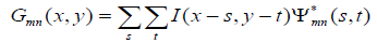
The discrete Gabor wavelet transform for a given image, I(x, y) is obtained by convolution using the following relationship [22]:
 (1)
(1)
where,
s and t are filter mask size variables,
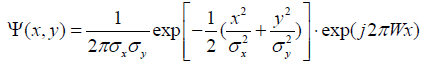
Ψ*mn is the complex conjugate of mn Ψmn , which is a class of selfsimilar functions generated from dilation and rotation of the following mother wavelet:
 (2)
(2)
where,
W is a modulation frequency.
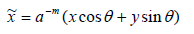
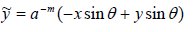
The self-similar Gabor wavelets are obtained using the following relationship:
 (3)
(3)
 (4)
(4)
where,
 (5)
(5)
and,
m=0, 1,…, M–1 specifies the scale
n=0, 1,…, N–1 specifies the orientation of the wavelet
M is the number of scales
N is the number of orientations
a is greater than 1, and represents a scale factor and is dependent on the higher center frequency and lower center frequency of interest θ = nπ / N.
After applying the Gabor filters on an image, an array of magnitudes is obtained. This contains the means and standard deviations that represent the texture feature components. Texture features are extracted using the Gabor filters. These filters use scales and orientations to provide additional views of a specific image. The total number of filters used on the image is equal the product of S and K (S*K); where, S represents the total number of scales and K represents the number of orientations. The texture feature vector for the image is constructed from the means and standard deviations obtained from each of the S*K views produced by the Gabor filters [19]. Figure 2 shows the optimal Gabor filters using Fisher’s linear discriminant (FLD) measure.

Figure 2: Optimal Gabor filters using FLD measure.ww
For this case, four scales and six orientations can be used. Different combinations have been tested and the parameters with the optimal results were chosen. A total of 24 views are used, which result in 24 means and 24 standard deviations for each sub-image. In the feature vector, the first 48 components are the texture features.
Color features
Color is an important dimension of human visual perception as it helps to recognize and discriminate visual content. Color features have been found to be effective for indexing and searching for color images, and these features can be extracted and matched easily [23]. The most common color metric used in the literature is the color histogram.
Each histogram bin is represented by a range of colors and the color histogram represents the coarse distribution of the colors in the image [24]. So, if two colors are in the same bin they are treated as similar colors. On the other hand, if two colors are in different bins they are considered different, even if they might be very similar to each other. By mapping the image to an appropriate color space, quantizing the mapped image and then counting the occurrence of each color, the color histogram for the image can be obtained.
By using the color histogram, similarity of color features can be specified by counting the color intensities. Any color could be reproduced by combining the three primary colors: red (R), green (G), and blue (B). Therefore, these three colors represent colors as vectors in 3D RGB color space. A color descriptor metric, such as the histogram, provides a way to quantify the similarity of color features in images by counting the color intensities. In general, a color image has three layers (R, G, and B); therefore, three color histograms with twelve bins being calculated for each sub-image. Thus, the next 36 features in the feature vector are related to color features.
Histogram of gradient (HOG)
Histogram of gradient representation (HOG) is used for capturing gradient structure. HOG computes gradients in regions and puts them in bins according to orientation [25]. HOG also computes the discretized gradients using 1-D centered point discrete derivative mask in both the horizontal and vertical directions. The vectors are given as,
 (6)
(6)
The region is then segmented into eight by eight cells. For each cell, a histogram of gradients is computed. For each pixel, a vote is cast that is weighted by the gradient magnitude and orientation. Each vote is cast toward a certain gradient orientation range corresponding to a bin in the histogram. The number of bins is 36 for each cell. Finally, each histogram is contrast normalized over spatial neighbors.
For each image after normalizing color, the indirect gradient is extracted for each cell. Each pixel within the cell votes for an oriented based histogram bin based on the values found in the gradient computation. For each cell, 36 bins are specified. In this case, after decomposing an image into 24 × 24 pixels cell, HOG dimension is 3500. Figure 3 shows the HOG representation of images from levee, grassland and mountain.

Figure 3: HOG representation for levee, grassland, and mountain.
Methods
A set of features consisting of local gradients and global color and texture features are extracted, which are used for scene recognition. Figure 4 shows the overview of this fully automated framework for identifying the scene of the image. For those images that were classified as levee the second phase is used to detect soil erosion.

Figure 4: Framework.
Analysis methodology
The objective of this work is to be able to classify the scene of an image using a set of training data. The image dataset, which is being used in this study, consists of images related to scenes where erosion can happen, such as along a levee. For this paper, a case study area was selected in the California central valley. 120 images were captured using drone aerial photography from scales that range from 2-5 meters from the ground. The images can be classified in six different scenes: levees, mountains, forest, degraded forest, grassland, or orchard. For evaluation purposes, the dataset is divided into training and testing; and different classification methods such as SVM, Naïve Bayes, Decision Trees, and Bootstrap Aggregation are used to perform the analysis.
A feature vector is extracted for each image. This feature vector is a combination of texture, color, and HOG features. Waikato Environment for Knowledge Analysis (WEKA) [26] will be used to apply classification methods, such as Naïve Bayes, Support Vector Machines, and Decision Trees. WEKA is a machine learning software with a collection of machine learning algorithms for data mining tasks. After the features have been extracted, a model is trained to detect the scene of each image. In the classification process, LibSVM, Decision Tree, Naïve Bayes, and Bootstrap Aggregation classifiers are used.
As discussed before, there are six scene classes: levee slope, mountains, forest, degraded forest, grassland, or orchard. For evaluation, the corpus will be divided into two sections: one section for training purposes and the other section for testing purposes. The training set consists of 80% of the corpus and testing consists of the remaining 20%. 10-Fold cross validation will be performed to increase the accuracy of the result.
In the second phase of this ongoing study after the scene of the image has been detected, the image is fed into a second image processing algorithm to detect erosion. The process entails using levee site photographs from before and after a rain event, or from a regular scheduled survey. The photographs can then be processed to determine the extent of change in surface texture. When certain benchmarks have been exceeded, mitigation work can be ordered to avoid catastrophic erosion, or excessive siltation that can lead to costly cleanups of the waterway; or in some cases, rain water might have to be discharged to nearby waterways resulting in costly flooding and environmental cleanups. The main goal of the work presented in this paper is to provide an overview of an algorithm that can be used to identify erosion problems along levees before they have adverse impacts on the environment; thus, avoiding costly flooding and cleanups that result from delayed erosion control.
Results
In the first phase of this study the image is classified into the following six scene classes: levee slope, mountains, forest, degraded forest, cropland, grassland or orchard. For each image a set of features consisting local gradients and global color and texture features are extracted and used to detect the scene. Table 1 shows the classification results (Tables 1 and 2).
| Scene Class | Precision | Recall | F-measure |
|---|---|---|---|
| Levee slope | 0.894737 | 0.85 | 0.871795 |
| Mountain | 0.823529 | 0.7 | 0.756757 |
| Forest | 0.625 | 0.75 | 0.681818 |
| Degraded forest | 0.666667 | 0.7 | 0.682927 |
| Grassland | 0.736842 | 0.7 | 0.717949 |
| Orchard | 0.85 | 0.85 | 0.85 |
Table 1: Classification results.
| Classified as Actual class | Levee slope | Mountain | Forest | Degraded forest | Grassland | Orchard |
|---|---|---|---|---|---|---|
| Levee slope | 17 | 2 | 0 | 1 | 0 | 0 |
| Mountain | 1 | 14 | 1 | 1 | 1 | 2 |
| Forest | 0 | 0 | 15 | 3 | 2 | 0 |
| Degraded forest | 0 | 0 | 6 | 14 | 0 | 0 |
| Grassland | 1 | 1 | 2 | 1 | 14 | 1 |
| Orchard | 0 | 0 | 0 | 1 | 2 | 17 |
Table 2: Confusion matrix.
By looking at the result and the confusion matrix, it can be seen that forest and degraded forest tend to get misclassified. Since we are using global images for each scene and the features consist of color and texture features, images with the same correlation, contrast, homogeneity, and same range of colors tend to be classified in the same category.
In the next phase, the images that were classified as levee site will be fed into another image processing algorithm to detect erosion. The algorithm is used to detect any major changes in surface texture by calculating the erosion surface area. Figure 5 shows the feature output of our erosion detection algorithm. In cases where before and after photos were available the algorithm generates all the erosion lines and compares the difference between width, height and number of lines. Any major changes are labeled as erosion.

Figure 5: Erosion detection output image and features.
Conclusions and Future Work
In this paper, we presented a two phase image processing algorithm that first detects the scene of the image and classifies it into 6 predefined classes. In the second phase of the algorithm, soil erosion is detected along a levee by generating global features along with local gradients and using supervised classification methods. Most erosion detection algorithms available require human observations and manual work, which is time consuming and error-prone. Other algorithms consist of a combination of field related work along with a high level of automation. What distinguishes the approach outlined in this paper with the state-of-the-art methods is the fact that the proposed methodology is fully automated and can detect areas highly prone to soil erosion from Landsat and aerial images taken using areal drones.
In this method the scene of the image is detected, which will help narrow the search space. The image processing model proposed can be used at a preprocessing stage to detect soil erosion along levees and avoid costly flooding and cleanups from delayed erosion control.
Quantifying erosion can be done using Terrestrial Laser Scanning (TSL). This method is widely used in geosciences but has some limitations in erosion detection. These limitations include accuracy of measurements and instability of the references used on steep slopes with near vertical viewing direction, on very small plots, or at locations where erosion magnitudes are very large. For the next phase of our study we are planning to use an emerging new equipment, Light Detection and Ranging (LIDAR). The scanner integrates a GPS receiver able to correlate individual scans and snitch them with accuracy up to ± 1 mm, with a 350-meter range.
References
- Rose CW (1985)Â Developments in soil erosion and deposition models. Adv Soil Sci 2: 1-63.
- Dewan A, Corner R, Saleem A, Rahman MM, Haider MR, et al. (2017) Assessing channel changes of the Ganges-Padma River system in Bangladesh using Landsat and hydrological data. Geomorphology 276: 257-279.
- Yao Z, Ta W, Jia X, Xiao J (2011) Bank erosion and accretion along the Ningxia–Inner Mongolia reaches of the Yellow River from 1958 to 2008. Geomorphology 127: 99-106.
- Kummu M, Lu XX, Rasphone A, Sarkkula J, Koponen J (2008) Riverbank changes along the Mekong River: remote sensing detection in the Vientiane–Nong Khai area. Quat Int 186: 100-112
- Sanyal J (2017) Predicting possible effects of dams on downstream river bed changes of a Himalayan river with morphodynamic modelling. Quat Int 453: 48-62.
- Nawfee SM, Dewan A, Rashid T (2018) Integrating subsurface stratigraphic records with satellite images to investigate channel change and bar evolution: a case study of the Padma River, Bangladesh. Environ Earth Sci 77: 89.
- Mallepudi SA, Calix RA, Knapp GM (2011) Material classification and automatic content enrichment of images using supervised learning and knowledge bases.
- Choung Y (2014) Mapping levees using LiDAR Data and Multispectral Orthoimages in the Nakdong River Basins, South Korea. Remote Sens 6: 8696-8717.
- Filin S, Goldshleger N, Abergel S, Arav R (2013) Robust erosion measurement in agricultural fields by colour image processing and image measurement. Eur J Soil Sci 64: 80-91.
- Iranmanesh F, Charkhabi AH, Jalali N, Ghafari AR (2004) Change Detection of Gully Erosion Using Image Processing in Dashtyari Region- Chabahar. FAO: Soil Conservation and Watershed Management Reseach Institute.
- Mulhem P, Leow WK, Lee YK (2001) Fuzzy conceptual graphs for matching images of natural scenes. To appear in IJCAI, pp. 1-6.
- Oliva A, Torralba A (2006) Building the gist of a scene: The role of global image features in recognition. Progress in brain research 155: 23-36.
- Lipson P, Grimson E, Sinha P (1997) Configuration based scene classification and image indexing. pp. 1007-1013.
- Carson C, Belongie S, Greenspan H, Malik J (2002) Blobworld: Image segmentation using expectation-maximization and its application to image querying. IEEE Transactions on Pattern Analysis and Machine Intelligence 24: 1026-1038.
- Li LJ, Socher R, Fei-Fei L (2009) Towards total scene understanding: Classification, annotation and segmentation in an automatic framework. pp. 2036-2043.
- Quattoni, Torralba A (2009) Recognizing Indoor Scenes. IEEE Conference on Computer Vision and Pattern Recognition.
- Tamura H, Mori S, Yamawaki T (1978) Textural features corresponding to visual perception. IEEE Transactions on Systems, Man and Cybernetics 8: 460-473.
- Zhang D, Lu G, Wong A, Indrawan M (2000) Content-based image retrieval using Gabor texture features In proceedings of 1st IEEE Pacific Rim conference on Multimedia (PCM), pp. 392-395.
- Li CS, Smith JR, Castelli V, Bergman LD (1998) Comparing texture feature sets for retrieving core images in petroleum applications. Proc. SPIE 3656, Storage and Retrieval for Image and Video Databases VII pp. 2-11.
- Manjunath BS, Ma WY (1996) Texture features for browsing and retrieval of Image data. IEEE Transactions on Pattern Analysis and Machine Intelligence 18: 837-842.
- Chen L, Lu G, Zhang D (2004) Effects of Different Gabor Filter Parameters on Image Retrieval by Texture. International Conference on Multimedia Modeling, pp. 273.
- Han J, Ma K (2002) Fuzzy Color Histogram and its Use in Color Image Retrieval. IEEE Transactions on Image Processing 11: 944-952.
- Dalal N, Triggs B (2005) Histograms of Oriented Gradients for Human Detection. IEEE Computer Society Conference on Computer Vision and Pattern Recognition pp. 886-893.
- Faloutsos, Taubin G (1993) The QBIC Project: Querying Images by Content Using Color, Texture and Shape. Proceedings SPIE 1908, Storage and Retrieval for Image and Video Databases 173-187.
- Bouckaert RR, Frank E, Hall MA, Holmes G, Pfahringer B, et al. (2010) WEKA-experiences with a java open-source project. J Machine Learn Res 11: 2533-2541.
Citation: Khazaeli M, Javadpour L, Estrada H, Takbiri-Borujeni A (2018) Assessment of Levee Erosion Using Image Processing and Contextual Cueing. J Ecosys Ecograph 8: 255.
Copyright: © 2018 Khazaeli M, et al. This is an open-access article distributed under the terms of the Creative Commons Attribution License, which permits unrestricted use, distribution, and reproduction in any medium, provided the original author and source are credited.
Share This Article
Recommended Journals
Open Access Journals
Article Usage
- Total views: 3231
- [From(publication date): 0-2018 - Mar 09, 2025]
- Breakdown by view type
- HTML page views: 2509
- PDF downloads: 722