Application of Remote Sensing for Evaluation of Land Use Change Responses on Hydrology of Muga Watershed, Abbay River Basin, Ethiopia
Received: 16-Aug-2018 / Accepted Date: 15-Oct-2018 / Published Date: 22-Oct-2018 DOI: 10.4172/2157-7617.1000493
Keywords: SWAT model; LU change; Muga watershed; ERDAS; Imagine; Catchment hydrology
Introduction
Watershed hydrology is affected by vegetation types, soil properties, geology, terrain, climate, land use practices, and spatial patterns of interactions among the different factors [1-4]. Land use changes are one of the main human induced activities altering the hydrological system [5]. The impacts of these land use changes become globally significant through their accumulative effects [6]. The intense human utilization of land resources has resulted in significant changes of the land use [7]. The increase in population has led to plot sub-divisions and competition for arable land. The competition for land has also ensured that other land uses within the sub-catchment, such as forestry, have come into direct competition with agriculture [8]. Human induced activities in the Muga watershed affect the catchment hydrology, which alter the surface runoff and reducing the ground water flow i.e., infiltration, percolation. This is happened due to the expansion of agricultural lands and decreasing of grasslands, forest and shrub lands. This study aims on application of SWAT model on the assessment of land use impacts on watershed hydrology and best scenarios suggested to address the problem of hydrological degradation.
Objectives of the study
The general objective of the study is to evaluate land use change responses on catchment hydrology of Muga watershed by using remote sensing technology. Moreover, this research tried to address the following specific objectives:
• To investigate the impact of land use change responses on hydrology of the watershed.
• To estimate runoff from the watershed using SWAT model.
• To evaluate the performance of SWAT model.
• To suggest best land use scenario for effective water resource management.
Description of the Study Area
Muga watershed (study area) is found in Upper Blue Nile Basin, which is about 248 km far from North West of Addis Ababa between the towns of Dejen and Bichena. This area is one of the choke mountain watershed which is located in the northern highlands of Ethiopia, within 10°6’30’’North to 10°43’30’’North and 37°49’00’’East to 38°16’30’’East. It covers an area of 641 km2. Muga River originates from Bibugn district near Choke Mountain at elevation of 4084 m.a.s.l and drains to Abbay River. The agro-climatic zone of Muga is wet/moist dega (temperate like climate-highlands with 2500-3000 meters altitude) and kola (hot and arid type, less than 1500m in altitude) when it reaches to Blue Nile River [9]. The dry season occurs between October and May while the wet season occurs mostly between June and September when the ICTZ is to the north of the country. The study areas have mean annual rainfall of 1445 mm, and the minimum and maximum temperature of the watershed is 5°C and 25°C respectively. Soil groups which are found in the study area are Eutric Vertisols (52.73%), Eutric Cambisols (17.07%), Eutric Leptosols (3.74%), Haplic Luvisols (11.34%), Haplic Nitosols (9.12%), Rendizic Leptosols (5.99%) and Urban (0.01%) (Figure 1).

Figure 1: Location of Muga watershed.
Research Methodology
During this study SWAT model was embedded in ArcGIS 9.3 to evaluate the impact of land use land cover change on hydrology of the watershed. ERDAS IMAGINE were also used for preliminary data processing, extracting, mosaicking of satellite images and image classification. The performances of SWAT model were evaluated using statistical measures to determine the quality and reliability of predictions when compared to observed values. Coefficient of determination (R2), Nash-Sutcliffe simulation efficiency (NSE), observations standard deviation ratio (RSR) and percent bias (PBIAS) were used for the goodness fit measures to evaluate the model prediction.
Application of remote sensing on land use changes
The information about land use change which is extracted from remotely sensed data is vital for updating land use maps and the management of natural resources and monitoring phenomena. The importance of land use mapping is to show the land use changes in the watershed area and to divide the land use in different classes of land use [10]. Remotely sensed imagery play a great role for obtaining information about the temporal trends and spatial distribution of watershed areas, and changes over the time dimension for projecting land use changes [11].
Overview of SWAT model
SWAT is a physically based, computationally efficient, and capable of simulating a high level of spatial detail by allowing the divisions of watersheds into smaller sub watersheds [12]. This model also plays a major role in analyzing the impact of land management practices on water, sediment, and agricultural chemical yields in large complex watersheds [13,14].
The hydrological component of the SWAT model
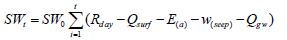
In SWAT, a watershed is divided into multiple sub-watersheds which are then further subdivided into Hydrological Response Units (HRUs) that consist of homogeneous land use, management, and soil characteristics. In the land phase process of the hydrological cycle, SWAT simulates the hydrological cycle based on the water balance of the soil profile.
 (1)
(1)
where, SWt, is the final soil water content (mm), SW0 is the initial soil water content (mm), t is the time (days), Rday is the amount of precipitation on day i (mm), Qsurf is the amount of surface runoff on day i (mm), Ea, is the amount of evapotranspiration on day i (mm), Wrchrg is the amount of water giving recharge to groundwater (shallow and deep aquifer) from the soil profile on day i (mm) and Qgw is the amount of groundwater flow on day i (mm).
SWAT offers two methods for estimating surface runoff: the SCS curve number procedure [15] and the Green and Ampt infiltration method [16]. Using daily or sub daily rainfall, SWAT simulates surface runoff volumes and peak runoff rates for each HRU. In this study, the SCS curve number method were used to estimate surface runoff because of the unavailability of sub daily data for Green & Ampt method. The SCS curve number equation is:
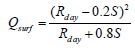
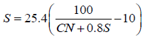
In which, Qsurf is the accumulated runoff or rainfall excess (mm), is the rainfall depth for the day (mm), S is the retention parameter (mm). The retention parameter is defined by equation 3.
Model input
SWAT is highly data intensive model that requires specific information about the watershed such as topography, land use, soil properties, weather data, and other land management practices.
Digital elevation model: DEM well define the topography of the area by describing the elevation of any point at a given location and specific spatial resolution as a digital file. The raw DEM was obtained Ministry of Water, Irrigation and Electricity (MoWIE) of Ethiopia with 90 m x 90 m resolution and projected using Arc GIS 9.3 software package; and used to delineate the watershed. Drainage pattern, slope, channel width and stream length with in the watershed was processed using DEM (Figure 2).

Figure 2: Digital elevation model of Muga watershed.
Land use land cover data: Land use is one of the highly influencing hydrological properties of the watersheds and it is very essential SWAT input for determining the watershed characteristics, and also used for comparison of impacts on the hydrology of the watershed. For land use classification process, 1986 and 2009 satellite images were downloaded from USGS/GLOVIS website and land cover maps had been prepared by using maximum likelihood supervised classification algorism of ERDAS IMAGINE software.
Soil data: World soil classification is developed by the Food and Agricultural Organization (FAO) that helped to generalize the soil pedogenesis in relation to the interaction with the main soil forming factors. Soil data was taken from the Ministry of Water, Irrigation and Electricity (MoWIE) of Ethiopia.
Weather data: SWAT model largely depends on meteorological data such as daily precipitation, maximum and minimum temperature, wind speed, relative humidity and solar radiation. The meteorological data was obtained from National Meteorological Agency (NMA) of Ethiopia. The climate data used for this study covers 26 years from January first, 1986 to December last, 2010 for six stations of Debre Markos, Mota, Yetnora, Yetmen, Bichena and Abbay sheleko (a place of meteorological station). The SWAT weather generator parameters were estimated using pcpSTAT (rainfall parameter calculator) and dew point temperature calculator Dew-02 [17]. The consistency of meteorological data was checked using double mass curve (Figure 3).

Figure 3: Digital elevation model of Muga watershed.
River discharge data: Daily flow data is required for SWAT calibration and validation of the simulated flow. Twenty-six daily flow data for Muga River near Yetmen Town was obtained from Ministry of Water, Irrigation and Electricity (MoWIE) of Ethiopia.
Model setup
In this model set up the following steps were followed: Data preparation, watershed delineation, HRUs definition, weather write up, SWAT simulation, sensitivity analysis, calibration and validation. The collected DEM was projected to UTM 37N. The satellite image was also classified using ERDAS Imagine and saved to raster data format (UTM 37N). Following DEM data preparation, watershed delineation proceeded using the projected 90 m by 90 m DEM. After watershed delineation, HRU definition was performed using multiple HRU classes of 10% land use, 10% soil and 5% slope discretization. SWAT simulation was also done using the HRUs and weather data inputs. Sensitivity analysis was also done using 26 years recorded river flow for identifying the most sensitive parameters. Calibration of flow simulations performed using the identified sensitive parameters for the periods 1989–1996 since the flow has no missing values during the record period. After a while, validation was done for the periods 2004–2007.
Global sensitivity analysis performs the sensitivity of one parameter while the value of other related parameters are also changing. Global sensitivity analysis uses t-test and p-values to determine the sensitivity of each parameter. The t-stat provides a measure of the sensitivity (larger in absolute values are more sensitive) and the p-values determine the significance of the sensitivity. A p-value close to zero has more significance. This type of sensitivity can be performed after iteration. The main problem related to global sensitivity analysis is that it needs a large number of simulations.
Model calibration is an effort to better parameterize a model to a given set of local conditions, thereby reducing the prediction uncertainty. Model calibration is performed by carefully selecting values for model input parameters (within their respective uncertainty ranges) by comparing model predictions (output) for a given set of assumed conditions with observed data for the same conditions.
After calibration, a validation procedure should be done to assess the performance of the calibrated parameters for an independent set of data in a different time period, with no further adjustment of parameters. Model validation is the process of demonstrating that a given sitespecific model is capable of making sufficiently accurate predictions.
SWAT-CUP (Calibration and Uncertainty Programs) was used for calibration and uncertainty analysis on stream flow parameters. SWAT-CUP is a public domain computer program for calibration of SWAT models. It links Generalized Likelihood Uncertainty Estimation (GLUE), Parameter Solution (Parasol), Sequential Uncertainty Fitting, ver. 2 (SUFI-2), Markov Chain Monte Carlo (MCMC) and Particle Swarm Optimization (PSO) procedures to SWAT output files. It enables sensitivity analysis, calibration, validation, and uncertainty analysis of a SWAT model.
The model performance was evaluated using Nash Sutcliff Efficiency (NSE), coefficient of determination (R2), observations standard deviation ratio (RSR) and percent bias (PBIAS).
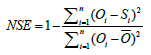
Nash–Sutcliffe efficiency (NSE): This statistic determines the relative magnitude of the residual variance compared to the observed data variance. NSE ranges from -∞ to 1, where 1 denotes perfect agreement between simulated and observed variables. NSE is formulated as:
 (4)
(4)
R2 ranges from 0 (which indicates the model is poor) to 1 (which indicates the model is good), with higher values indicating less error variance, and typical values greater than 0.6 are considered acceptable [18]. The R2 is calculated using the following equation:
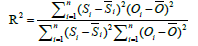 (5)
(5)
RMSE observations standard deviation ratio (RSR): RSR standardizes the root mean square error (RMSE) using the observation standard deviations. It is calculated as:
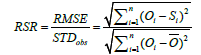 (6)
(6)
Percent Bias (PBIAS): PBIAS is a measure of how much (in percentage) the observed variable is either underestimated or overestimated. It is calculated as shown:
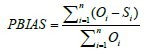 (7)
(7)
Where O ̅ is the average measured discharge, Si is the simulated discharge for each time step, Oi is the observed discharge value, and S ̅ is the average simulated value, n is the total number of values within the period of analysis, RMSE is the root mean square error, STDobs is the standard deviation of the observed variable (Table 1). The scenario analysis was done based on the land use map of 2009, in which the land use was modified and run the model. The analysis was done by changing three land use types into forest with 5% for each, i.e., agriculture to forest, grass land to forest and shrub land to forest; hence, the best land use land cover change scenario was suggested.
| Performance rating | NSE | RSR | PBIAS (%) |
|---|---|---|---|
| Very good | 0.75 < NSE ≤ 1.00 | 0.00 ≤ RSR ≤ 0.50 | PBIAS < ± 10 |
| Good | 0.65 < NSE ≤ 0.75 | 0.50 < RSR ≤ 0.60 | ± 10 ≤ PBIAS < ± 15 |
| Satisfactory | 0.50 < NSE ≤ 0.65 | 0.60 < RSR ≤ 0.70 | ± 15 ≤ PBIAS < ± 25 |
| Unsatisfactory | NSE ≤ 0.50 | RSR > 0.70 | PBIAS ≥ ± 25 |
Notes: *PBIAS: Percent Bias; RSR: RMSE Observation Standard Deviation Ratio; NSE: Nash-Sutcliffe Efficiency.
Table 1: General performance rating for recommended statistics for monthly time step.
Result and Discussion
Land use change analysis
After through step by step processing and land use detection the map showing six (cultivated, water, grass land, shrub land, urban and forest) classes of land use were created unifying these classes for the 1986 and 2009. Afterwards, spatial analysis of land use has been performed to describe the overall land use patterns through the watershed. Generally, major parts of cultivated land found at the middle and south eastern parts of the watershed, grasslands at north and southwestern, while shrub lands at north eastern parts of the watershed (Figure 4). An accuracy of image classification was checked using 41 randomly selected control points. The accuracy assessment was performed by using classified land use maps, ground truth points and Google Earth. The 2009 land use classification has showed, user’s accuracy and producer’s accuracy are greater than 85%, as well the overall accuracy of 89.38% (Table 2). These indicate the land sat image classification is performed accurately. During this study periods (1986–2009); there had been a significant land use change in the watershed where the agricultural land had been increased from 40.01% to 76.47%, while grass lands were decreased from 46.23% to 10.99%. This could be attributed to the increase in population that has increased the demand for agricultural land in the watershed (Table 3). Muga watershed is densely populated with an annual growth rate of 2.31% and also the economic activity of the population is depends on agriculture and cattle breeding activities [19].

Figure 4: General framework of the methodology used.
| Reference Data | |||||||||
|---|---|---|---|---|---|---|---|---|---|
| Variables | Urban | Water | Forest | Grass Land | Cultivated Land | Shrub Land | Total | User’s Accuracy | |
| Classification Data | Urban | 43 | 0 | 0 | 1 | 0 | 0 | 44 | 97.72% |
| Water | 0 | 21 | 0 | 1 | 0 | 1 | 23 | 91.3% | |
| Forest | 0 | 2 | 60 | 1 | 2 | 2 | 67 | 89.55% | |
| Grass land | 1 | 0 | 2 | 24 | 1 | 0 | 28 | 85.71% | |
| Cultivated land |
2 | 1 | 0 | 0 | 43 | 0 | 48 | 89.58% | |
| Shrub land | 0 | 0 | 3 | 0 | 0 | 14 | 17 | 82.45% | |
| Total | 46 | 24 | 65 | 27 | 46 | 17 | 227 | 89.38% | |
| Producer’s Accuracy |
93.5% | 87.5% | 92.3% | 88.9% | 93.47% | 82.35% | Overall Accuracy | ||
Table 2: Confusion matrix for the land use classification of 2009.
| Land use classes | 1986 | 2009 | Land use change from 1986 to 2009 | |||
|---|---|---|---|---|---|---|
| Area (ha) | % | Area (ha) | % | Area (ha) | % | |
| Agricultural land | 25704.6 | 40.1 | 49018.3 | 76.47 | +23313.7 | +36.37 |
| Grassland | 29634.0 | 46.23 | 7044.7 | 10.99 | -22589.3 | -35.24 |
| Shrub land | 6903.7 | 10.77 | 6833.2 | 10.66 | -70.5 | -0.11 |
| Forest | 1230.7 | 1.92 | 448.7 | 0.7 | -782.0 | -1.22 |
| Water | 339.8 | 0.53 | 262.8 | 0.41 | -77.9 | -0.12 |
| Urban | 288.5 | 0.45 | 493.6 | 0.77 | +205.1 | +0.32 |
Table 3: Summary of land use change percentage of Muga watershed.
River flow modeling
Sensitivity analysis was performed for selecting of sensitive parameters which needs calibration. Twenty-six flow parameters were considered for sensitivity analysis using the observed flow data of Muga River gauge station; of which five flow parameters were identified sensitive. This implied that, the parameters have a significant influence on hydrology of the watershed.
In Muga watershed, SCS runoff curve number (CN2) was identified highly sensitive (Tables 4 and 5). The global sensitivity results for Muga watershed indicated (Table 5) that parameters having more negative t-stat value and more positive p-value were very sensitive parameters of flow. Calibration was done for sensitive flow parameters of SWAT with observed average monthly stream flow data. Manual calibration was performed for the simulated results based on the sensitive parameters. This was done by simulating the flow for eight years period from 1989– 1996.
| Parameters | Rank | Min | Max | Fitted Value | ||
|---|---|---|---|---|---|---|
| Name | Description | |||||
| R__CN2.mgt | SCS runoff curve number (%) | 1 | -25 | 25 | 0.08 | |
| V__ESCO.hru | Soil evaporation compensation factor | 2 | 0 | 1 | 0.75 | |
| V__GWQMN.gw | Threshold depth of water in the shallow aquifer required for return flow (mm) | 3 | 0 | 1000 | 120 | |
| V__CANMX.hru | Maximum canopy storage (mm H2O) | 4 | 0 | 10 | 8.5 | |
| R__SOL_AWC.sol | Soil available water capacity (water/mm soil) | 5 | -25 | 20 | 8 | |
Table 4: List of parameters and fitted values for monthly flow.
| Parameter name | t-Stat | P-value |
|---|---|---|
| R__CN2.mgt | -1.95 | 0.67 |
| V__ESCO.hru | -0.6 | 0.54 |
| V__GWQMN.gw | 0.64 | 0.29 |
| V__CANMX.hru | 1.55 | 0.01 |
| R__SOL_AWC.sol | 2.76 | 0.01 |
Table 5: Global sensitivity results for Muga watershed.
The result of calibration for monthly flow showed that there is a good agreement between the measured and simulated average monthly flows with Nash-Sutcliffe simulation efficiency (NSE) of 0.83, coefficient of determination (R2) of 0.89, observation standard deviation ratio (RSR) of 0.32 and percent bias (PBIAS) of -10.8% (Figure 5).

Figure 5: Land use map of year (a) 1986 and (b) 2009.
The model validation was also performed for four years from 2004 to 2007 without further adjustment of the calibrated parameters. The validation simulation also showed good agreement between the simulated and measured monthly flow with the Nash-Sutcliffe simulation efficiency (NSE) value of 0.79, coefficient of determination (R2) of 0.86, observation standard deviation ratio (RSR) of 0.54 and percent bias (PBIAS) of -19.8% (Figure 6).

Figure 6: Result of calibration for average monthly stream flow (1989-1996) for 1986 land use.
In general, the model performance assessment indicated that there is a good correlation between the monthly measured and simulated flows (Figure 7).

Figure 7: Result of validation for average monthly stream flow (2004-2007) for 1986 land use.
Evaluation of hydrological impacts due to land use land cover changes
After calibration and validation, SWAT was run using the two land use maps for the period of 1986 to 2009 while putting the other input variables the same for both simulations to quantify the variability of catchment hydrology due to the changes of land use. Surface flow, lateral flow and ground water flow change during two years were calculated and used as indicators to evaluate the effect of land use change on the catchment hydrology. Table 6 presents the mean annually surface flow, lateral flow and ground water flow for 1986 and 2009 land use maps and its variability (1986 -2009). As showed in Table 6, the contribution of surface flow has increased from 351.73 mm to 375.69 mm, lateral flow has decreased 96.85 mm to 91.47 mm whereas the ground water flow has decreased from 384.07 mm to 360.41 mm due to the land use change occurred between the periods of 1986 to 2009. Generally, surface runoff has increased throughout the study period for over 23 years period with a magnitude of 23.96 mm, while groundwater and lateral flow decreased with 23.66 mm and 5.38 mm respectively. These variations of hydrology were due to an increasing of cultivated land and decreasing of other land use types through study period. As indicated in Table 7, the mean monthly stream flow for wet months had increased by (+) 3.74 mm while decreased by (-) 1 for dry seasons mm during the 1986-2009 periods. This is due to expansion of agricultural land over grasslands, forests and shrub lands those results in the increase of surface runoff following rainfall events (Figure 8).

Figure 8: Mean annually surface runoff, lateral, groundwater flow and percolation variability (1986-2009).
| Mean monthly flow values (mm) | Mean monthly flow change from 1986 to 2009 |
||||
|---|---|---|---|---|---|
| Land use land cover 1986 | Land use land cover 2009 | ||||
| Wet months | Dry months | Wet months | Dry months | Wet months | Dry months |
| (Jun, Jul, Aug) | (Jan, Feb, Mar) | (Jun, Jul, Aug) | (Jan, Feb, Mar) | (Jun, Jul, Aug) | (Jan, Feb, Mar) |
| 254.24 | 8.05 | 257.98 | 7.05 | 3.74 | -1 |
Table 6: Mean monthly surface, lateral, groundwater flow and percolation and their variability during 1986-2009.
| Mean monthly flow values (mm) | Mean monthly flow change From 1986 to 2009 |
||||
|---|---|---|---|---|---|
| Land use land cover 1986 | Land use land cover 2009 | ||||
| Wet months | Dry months | Wet months | Dry months | Wet months | Dry months |
| (Jun, Jul, Aug) | (Jan, Feb, Mar) | (Jun, Jul, Aug) | (Jan, Feb, Mar) | (Jun, Jul, Aug) | (Jan, Feb, Mar) |
| 254.24 | 8.05 | 257.98 | 7.05 | 3.74 | -1 |
Table 7: Mean monthly wet and dry month's stream flow and their variability during 1986-2009.
Land use land cover change scenario analysis
By using land use land cover of 2009 as a reference, three scenarios were simulated to suggest best land use scenario. In scenario 1 (5% of cultivated land is changed to forest) the mean annual surface runoff is decreased from 375.69 mm to 351.36 mm, lateral flow and groundwater flow increased from 91.47 mm to 95.57 mm and 360.41 mm to 369.60 mm respectively. In scenario 2 (5% of grass land is changed to forest) mean annually surface runoff (SURQ) decreased from 375.69 mm to 357.69 mm, lateral flow and groundwater flow increased from 91.47 mm to 92.07 mm and 360.41 mm to 362.79 mm respectively. In scenario 3 (5% of shrub land is changed to forest) the mean annual surface runoff is decreased from 375.69 mm to 357.08 mm, lateral flow and groundwater flow increased from 91.47 mm to 91.70 mm and 360.41 mm to 361.38 mm respectively. All the scenarios worked have decreased surface runoff and increased groundwater and lateral flow. These scenarios are important suggestions to alleviate water degradation problem in the watershed. From the above scenarios discussed, scenario 1 is the best scenario to answer the objective as compared to others.
Conclusion
SWAT was applied to examine the long-term hydrological impact of land use change in the Muga watershed using a detailed land use record with a roughly 23-year interval classified based on Landsat images from 1986 to 2009. This model was calibrated and validated using observed stream flow data in 1989-1996 and 2004-2007 respectively, and then simulated using different land use scenarios in 1986-2010 to quantify the long-term hydrological impacts due to the land use change. The simulation results showed that land use land cover change was significantly alter the hydrologic response of Muga watershed. Infiltration was decreased in the watershed due to the expansion of agricultural lands from 1986 to 2009, which alter surface runoff. Understanding how the land use changes influence the sub-catchment hydrology will enable planners to formulate strategies to reduce undesirable effects of future land use changes. It is evident that the sub-catchment hydrology is currently under pressure following the rapid land use change which was taken place in Muga River. The study revealed that there are major land use land cover changes in Muga watershed for the period covered by the study, which are mainly associated with expansion of agricultural lands and deforestation. These changes had negative effects on the flow regime and recharge of Muga River. The results revealed that more land use changes are likely to take place as more land is converted over time especially forest and grasslands land to agricultural land, which threatens the existence of water sources in the future. The simulation of land use scenarios showed the impact that land use change have on the catchment hydrology and water components which all the scenarios increased the base flow and decreased surface runoff as compared to the land use of 2009. As discussed on the result and discussion part, scenario-1 (agricultural land to forest scenario) was best scenario for the objective. The stake holders and other concerned bodies can apply this best scenario to protect catchment hydrology degradation.
Acknowledgments
I am very grateful to thank Arba Minch Institute of Water Technology, and Ministry of Water, Irrigation and Eelectricity (MoWIE) for providing me meteorological and hydrological data freely.
Conflict of Interest
The authors declare that there are no conflicts of interest regarding the publication of this paper.
References
- Schulze RE (2000) Hydrological responses to land use and climate change: A southern African perspective, Ambio 29: 12-22.
- Zhang X, Srinivasan R, Hao F (2007) Predicting hydrologic response to climate change in the luohe river basin using the SWAT Model. ASABE 50: 901-910.
- Huang MB, Zhang L (2004) Hydrological responses to conservation practices in a catchment of the Loess Plateau, China, Hydrological Processes 18: 1885-1898.
- Brown AE, Zhang L, McMahon TA, Western AW, Vertessy RA (2005) A review of paired catchment studies for determining changes in water yield resulting from alterations in vegetation. Journal of Hydrology 310: 28-61
- Calder IR (1998) Water-resource and land use issues. SWIM Paper 3. Colombo: IIMI.
- Turner BL, MeyerWB (1994) Changes in land use and land cover: A global perspective. Cambridge: Cambridge University Press. New York, USA.
- Bronstert A, Niehoff D, Burger G (2002) Effects of climate and land-use change on storm runoff generation: Present Knowledge and modelling capabilities. Hydrol Process 16: 509-529.
- Lambin EF, Geist HJ, Lepers E (2003) Dynamics of land use and land cover change in tropical regions. Annu. Rev. Environ. Resour 28: 205-241.
- NMSA (2001) Initial National Communication of Ethiopia to the United Nations Framework Convention on Climate Change (UNFCCC) National Meteorological Service Agency, Addis Ababa, Ethiopia.
- William BM, Billie LT (1991) Changes in land use and land cover: A global perspective. University Corporation of America Office for Interdisciplinary Earth Studies, Cambridge University Press, USA.
- Atasoy M, Biyik C, Ayaz, H, Karsli F, Demir O, et al. (2006) Monitoring land use changes and determining the suitability of land for different uses with digital Photogrammetry. Remote Sensing and Photogrammetry, Cairo, Egypt. 23: 712-721
- Gassman PW, Reyes MR, Green CH, Arnold JG (2007) The soil and water assessment tool: Historical development, applications, and future research directions. Trans. ASABE 50: 1211-1250.
- Jaroslav MH, Marcel RS, Gresáka JB, Geografický SB (1996) Modeling spatial and temporal changes of soil water erosion. Geograficky casopis.
- Arnold JG, Fohrer N (2005) Current capabilities and research opportunities in applied watershed modeling. Hydrol. Process 19: 563-572.
- USDA Soil Conservation Service (SCS) (1972) National Engineering Handbook Section 4 Hydrology, Chapters 4-10.
- Green WH, Ampt GA (1911) Studies on soil physics. Part 1: The flow of air and water through soils J Agric Sci 4: 1-24.
- Santhi C, Arnold JG, Williams JR, Dugas WA, Srinivasan R, et al. (2001) Validation of the SWAT model on a large river basin with point and nonpoint sources, JAWRA 37: 5
- CSA (2008) Summary and statistical report of the 2007 population and Housing census: Population size by age and sex. Addis Ababa: Federal Democratic Republic of Ethiopia Population Census Commission.
Citation: Demeke GG, Andualem TG (2018) Application of Remote Sensing for Evaluation of Land Use Change Responses on Hydrology of Muga Watershed, Abbay River Basin, Ethiopia. J Earth Sci Clim Change 9: 493. DOI: 10.4172/2157-7617.1000493
Copyright: © 2018 Demeke GG, et al. This is an open-access article distributed under the terms of the Creative Commons Attribution License, which permits unrestricted use, distribution, and reproduction in any medium, provided the original author and source are credited.
Share This Article
Recommended Journals
Open Access Journals
Article Tools
Article Usage
- Total views: 3752
- [From(publication date): 0-2018 - Feb 22, 2025]
- Breakdown by view type
- HTML page views: 2996
- PDF downloads: 756