Research Article Open Access
Analytical Approach to Calculate the Heat Fluxes in the Atmosphere and to Quantify the Sensitivity of Earth Temperature due to CO2 and H2O
Tino Redemann* and Eckehard Specht
Otto von Guericke University, Institute of Fluid Dynamics and Thermodynamics, Magdeburg, Germany
- *Corresponding Author:
- Redemann T
Otto von Guericke University
Institute of Fluid Dynamics and Thermodynamics
39106 Magdeburg, Germany
Tel: +49-391-67-58125
E-mail: tino.redemann@ovgu.de
Received April 21, 2016; Accepted May 17, 2016; Published May 25, 2016
Citation: Redemann T, Specht E (2016) Analytical Approach to Calculate the Heat Fluxes in the Atmosphere and to Quantify the Sensitivity of Earth Temperature due to CO2 and H2O. J Ecosys Ecograph S5: 012. doi:10.4172/2157-7625.S5-012
Copyright: © 2016 Redemann T, et al. This is an open-access article distributed under the terms of the Creative Commons Attribution License, which permits unrestricted use, distribution, and reproduction in any medium, provided the original author and source are credited.
Visit for more related articles at Journal of Ecosystem & Ecography
Abstract
A mathematical model has been developed to understand the effect of carbon dioxide and water vapor on the mechanism of global warming. First, the increase of the CO2 concentration in the atmosphere could be based on the anthropogenic CO2 emissions according to the combustion of fossil fuels. Second, the heat fluxes in the atmosphere were described by known relations in thermal engineering. Here, the heat transfer due to radiation between the gas which contains water vapor and carbon dioxide, and the Earth's surface as well as the clouds is considered. The emissivity of the gases depends on temperature, and the gas concentration and the beam length of the atmospheric layer. The sensitivity of this model was quantified less, when e.g. the cloud height and the relative humidity of the atmosphere were varied. The known average temperature of the Earth was used to validate this model. The temperature of the Earth increases significantly with the CO2 concentration. When the concentration of CO2 is doubled, the temperature of the Earth increases by 0.43 K.
Keywords
Global warming; Carbon dioxide; Heat transfer; Radiation; Climate sensitivity
Nomenclature
| Symbol | Meaning | Unit |
|---|---|---|
| A | Area | m2 |
| E | Energy turnover | J/s |
| M | Mass | kg |
| Mass flow rate | kg s-1 | |
| Molar mass | kg mol-1 | |
| R | Resistance | - |
| RH20 | Gas constant of water vapor e.g. | J kg-1 K-1 |
| RI | Heat exchange resistance between Earth and clouds | - |
| T | Temperature | °C, K |
| c | Concentration, mole fraction | - |
| Emissive power | W m-2 | |
| g | Gravity | m s-2 |
| Brightness | W m-2 | |
| k | Number of resistances | - |
| p | Total pressure, partial pressure | Pa |
| Heat flux | W m-2 | |
| s | Beam length | m |
| t | Time | s |
| x | Specific emissions | kg J-1 |
| z | Height, altitude | m |
| Enthalphy change | J kg-1 | |
| Emissivity | - | |
| View factor | - | |
| Relative humidity | - | |
| Stefan-Boltzmann constant | W m-2 K-4 |
| Index | Meaning |
|---|---|
| 0 | Standard conditions |
| Space | |
| C | Clouds |
| CON | Convection |
| E | Earth |
| G | Gas |
| I | Heat exchange resistancebetween Earth and clouds e.g. |
| RAD | Radiation |
| SO | Solar |
| VAP | Vaporization |
| b | Black body |
| s | Saturated |
Introduction
Global warming is currently a widely discussed topic over which opinions vary greatly. On one hand, there are climatologists, who are convinced that global warming will lead to a climatological catastrophe. On the other hand, some references say that the temperature change is caused by natural climate fluctuations. Numerous multilayer models have already been developed to calculate the effects of human influence on the climate. These models are often very complex and difficult to comprehend due to the elusive discussion about the relation between the properties of the atmospheric layers and the radiative behavior of the involved gases such as water vapor and carbon dioxide [1].
Therefore, a simplified mathematical model was established in order to show how anthropogenic carbon dioxide affects the global temperature of the Earth. With this model, the mechanism of global warming caused by CO2 can be made understandable. Specifically, the focus is on the determination of the radiative gas properties using the temperature, gas concentration and beam length of the atmospheric layers defined through the model. Using this mode all heat fluxes in the atmosphere as well as the Earth surface temperature can be calculated. All other simplified models for global warming [2-4] calculate only special effects of global warming such as single radiative heat fluxes.
The description of complex processes using simplified mathematical models is a common practice in industrial engineering. That such models are limited in their accuracy is accepted in this context. Simplified models are necessary to make the principal effect of the influences comprehensible and to find a solution quickly. Such rapidly found solutions are only approximate solutions. When there is more time to solve the problem, a technical apparatus is simulated with complex, multidimensional mathematical models. Here, the highest possible accuracy of the results will be expected. Even complex mathematical models are only accepted in the industrial practice if they are validated with experimental results. If applicable, the models are adjusted to realistic conditions by choosing different parameters, for example, the heat transfer coefficient or the reaction coefficient [1].
An analogous approach is taken for the simulation of the influence of anthropogenic CO2 on global warming. For describing the mechanism of the greenhouse effect, it is sufficient to make the assumption that the Earth has a uniform temperature. Therefore, no distinction was made between land and oceans. The modeling of the green house effect in the atmosphere is similar to the modeling of thermal processes in industrial furnaces [1]. There are similar heat transfer mechanisms by radiation in the atmosphere. There is also a gas consisting of H2O and CO2 (the combustion gas) in the radiation exchange between bodies of different temperatures.
In order to evaluate the influence of anthropogenic CO2 Emissions  on global warming, the accumulation of CO2 in the atmosphere is described in the following section.
Anthropogenic CO2 emissions
The anthropogenic CO2 emissions are mainly traced back to the combustion of fossil fuels and can be estimated with
 (1)
(1)
where E is the converted energy amount of coal, oil and gas and xC02 the specific CO2 emissions per energy unit fuel. In 2013,
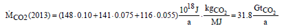 (2)
(2)
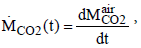
about 32 Gt CO2 were emitted in the atmosphere. The change of the total amount of CO2 in the atmosphere depends on the annual emissions and can be described with
 (3)
(3)
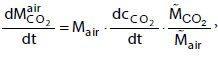
The temporal change of the CO2 concentration cC02 in the atmosphere can be obtained with the relation
 (4)
(4)
where Mair is the mass of the atmosphere and  is the molar mass of CO2 and air, respectively. The mass of the atmosphere is calculated from the balance of forces at the earth surface,
 (5)
(5)
where g is the acceleration of gravity, p0 is the standard pressure and AE is the surface area of the globe. In 2013, the increase of the CO2 concentration has to be 4 ppm due to the CO2 emissions named in equation (2).
In Figure 1, the measured CO2 concentration in the period from 1960 to 2015 is shown [5]. The monthly averaged data, as well as the yearly averaged data are shown in the figure. It can be seen that, since 2000, the CO2 concentration increases linearly at a rate of about 2 ppm per year. In comparison to the previous calculated value, only half of the anthropogenic CO2 emissions stay in the atmosphere and the rest has to be absorbed by vegetation and oceans.

Figure 1: Measured CO2 concentration in the atmosphere [5].
With the help of climate models, the temperature increase due to anthropogenic emissions of CO2 can be estimated. For the evaluation of its consequences on climate, the temperature increase is used, which is caused by a doubling of the CO2 concentration in the atmosphere. The year 1990 acts as reference year.
In the reference year 1990 the atmosphere contained about 355 ppm CO2. To make the impact on the earth’s temperature due to the doubling of the CO2 concentration visible, the heat flows in the atmosphere are considered in the following sections.
Global Energy Balance Earth-Atmosphere
Model for radiation and energy flows through the atmosphere
Radiation from the Sun is the only source of energy for the Earth. The heat flux from the Sun can be measured [1]. At the upper boundary of the atmosphere, the Earth receives a heat flow rate of 1368 W m-2. This parameter is named the extra-terrestrial solar constant. Since the cross sectional area of the Earth is only a quarter of its surface area, an average of 342 Watts is allotted to each square meter. The energy balance of the Earth and its atmosphere presented by Kiehl and Trenberth [6] is shown in Figure 2.

Figure 2: Heat fluxes in the atmosphere [courtesy of: Kiehl and Trenberth [6]].
About 30% of the short wave radiation from the Sun is reflected back into space by the atmosphere and the Earth’s surface. The ratio of the radiation reflected back by the Earth to the incident radiation is called albedo. Consequently, the heat flow rate is reduced to 235 W m-2. The clouds and the atmosphere absorb about 20% of the radiation and the remaining 50% is absorbed on the Earth’s surface (land, ocean). In thermal equilibrium, the energy supplied to the Earth must also be released. This occurs through the heat emission of the Earth’s surface, which amounts to 390 W m-2, under the assumption that the Earth is an ideal grey body. By comparing this heat emission with the Sun’s radiation, it becomes clear that the radiation of the Earth’s surface is higher. A part of this long wave radiation reaches Space directly through the atmospheric window (40 W m-2); the other part is absorbed by the atmosphere, clouds and greenhouse gases. Table 1 gives an overview of the most important greenhouse gases and their concentration in the atmosphere [5]. As shown in the Table, H2O and CO2 are the gases with the highest concentration in the atmosphere. The concentration of methane and nitrous oxide is substantially smaller [1].
| Gas | Concentration(2015) |
|---|---|
| Water vapor | variable 0-2% |
| Carbon dioxide | 399 ppm |
| Methane | 1838 ppb |
| Nitrous Oxide | 329 ppb |
Table 1: Greenhouse gases [5].
The greenhouse gases and clouds radiate 195 W m-2 into space and also yield a counter radiation of 324 W m-2 to the Earth’s surface. This causes a positive energy balance for the Earth’s surface and in the same proportion, a negative balance for the atmosphere. In order for the radiation balance to be equal to zero, equilibrium between the Earth’s surface and the atmosphere must be obtained. Therefore, the two heat fluxes, convection (24 W m-2) and evaporation (78 W m-2), are included in the energy balance. This description of the heat fluxes is found in many fields of climatology [1]. In the following section, this heat flow will be described with mathematical relationships in order to make the influence of CO2 clear.
Mathematical modeling
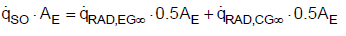
For the mathematical description of heat fluxes, the back radiation will not be included. Rather, the net heat fluxes exchanged according to the Stefan-Boltzmann law are considered as is usual in thermal engineering. The effective heat fluxes are summarized in Figure 3. About 50% of the Earth is covered with clouds [7,8]. The clouds as well as dust, aerosols, and a shortwave band of H2O in the atmosphere act as a radiation shield, meaning that the total radiation at the Earth’s surface is reduced. Consequently, the heat flow rate is reduced to 235 W m-2 as presented in Figure 2. In thermal equilibrium the solar radiation that reaches the Earth’s surface must be released into space [1]. One part of the heat is radiated through the cloud-free sky directly into space. The other part is transferred by radiation, convection and evaporation to the clouds. Therefore, the total heat flux can be described using
 (6)
(6)
Where,
 (7)
(7)
Subsequently, the clouds radiate the transferred heat fluxes through their upper surface into space. Neglecting other greenhouse gases, such as methane and nitrous oxide, because of their low concentrations allows discussion regarding the effect of CO2 and H2O in the atmosphere on the global warming separately. Absorption capacity, concentration and residence time of gases are used to evaluate the so called global warming potential. Indeed, methane and nitrous oxide have high global warming potential as well, but the reason for this is because of the long residence time in the atmosphere. Thus, the heat fluxes in the atmosphere are not significantly influenced.

Figure 3: Simplified description of the heat fluxes in the atmosphere.
Also, the model is simplified such that that the heat is transported without resistance through the clouds and the clouds thus have a uniform temperature.
The following equations are valid for the three heat fluxes by radiation:
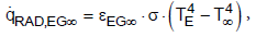 (8)
(8)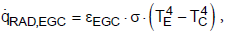 (9)
(9)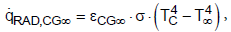 (10)
(10)
where TE, TC, T8 are the temperatures of the Earth, the clouds and of the space, eEG8, eEGC, eCG8 are the effective emissivities and s is the Stefan- Boltzmann constant (s = 5.67 × 10⁻⁸ W m-2 K-4).
On Earth, the average annual precipitation is 1000 mm m-2 a-1. This water quantity evaporates on the surface and condenses into clouds. The vaporization enthalpy of water of 2500 kJ kg-1 leads to a specific heat flux of  . The specific heat flux due to convection is according to Figure 2.
 , which corresponds to an average heat transfer coefficient of about 2 W m-2 K-1. This is a typical value for the free convection of horizontal plates [1]. The calculation of the radiative heat fluxes and the temperature of the Earth as well as the clouds will be discussed in the following chapter.
Heat transfer by radiation
Using the network method, the radiation exchange between two surfaces and a radiant gas can be calculated [9-11]. The network analogy for the Earth, gas, and cloud system is shown in Figure 4.

Figure 4: Equivalent circuit diagram for the radiation exchange.
For the total heat flow resulting between the vertices, Earth and clouds, the following equation is defined
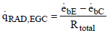 (11)
(11)
Where  and
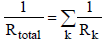
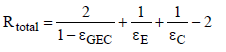
and  are the emissive power of the earth and the clouds as black bodies and Rtotal is the total resistance between earth and clouds. To calculate the total resistance, Kirchhoff’s Law from electrical engineering is used. If k resistances are connected in series, the individual resistances are summated as
  . For a parallel circuit of k resistances, the reciprocals of the resistances are summated as
In order to calculate the total resistance of the network shown in Figure 4, first the partial resistance RI is calculated, which occurs between the brightness point’s  and
and  . The resistances RGC and REG are connected in series and lie parallel to the resistance REC. Therefore, the partial resistance RI is given by equation (12)
 (12)
(12)
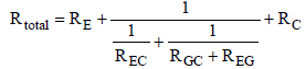
The total heat flux ![]() has to overcome the resistances RE, RI, and RC between Earth, gas and clouds. Since the three resistances are connected in series, the total resistance of the system is calculated through equation (13).
has to overcome the resistances RE, RI, and RC between Earth, gas and clouds. Since the three resistances are connected in series, the total resistance of the system is calculated through equation (13).
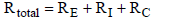 (13)
(13)
Equation (12) is substituted into equation (13), resulting in the following total resistance:
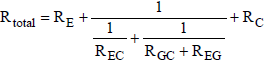 (14)
(14)
The surface resistances are given assuming grey radiation as:
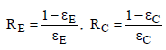 (15)
(15)
Where εE is the emissivity of the Earth and εC is the emissivity of the clouds. The radiation exchange resistances can be calculated as follows:
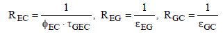 (16)
(16)
Here ƮGEC is the transmissivity of the gas, and εEG and εGC are the effective emissivities between gas and Earth or clouds respectively. Assuming grey gas behavior the transmissivity can be expressed by the emissivity ƮGEC = 1 − εGEC. Since the distance between the clouds and Earth is small compared to the Earth curvature, the view factor is determined φEC = 1. Considering the encountered assumptions, the total resistance can be calculated as follows:
 (17)
(17)
The emissive black power is given by
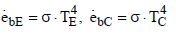 (18)
(18)
The heat flux can be expressed with the effective emissivity
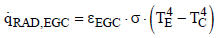 (19)
(19)
for which the following is obtained from Eq. (17)
 (20)
(20)
For the radiation of the clouds into space and of the Earth into space, the same mechanism can be employed. Since space is a black body (ε∞ = 1) it follows that:
 (21)
(21)
where

and
 (22)
(22)
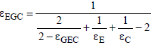
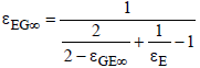
These two overall emissivities can be approximated by
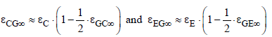 (23)
(23)
The two gas emissivities increase with CO2 concentration, as shown later. Therefore, the overall emissivities decrease. As a consequence, the temperatures according to equation (21) must increase because the heat flux is constant from the sun. That is the principal mechanism of global warming. Because of an increasing transport resistance for the heat flux the temperature must increase for compensating.
In the following section the required emissivities of the gases are calculated.
Determination of the emissivity of gases
Optical thickness: The emissivity of gases depends on the product of partial pressure and beam length as well as on the temperature. In the atmosphere, the temperature and the partial pressure decrease with higher altitude, so that suitable mean values must be determined.
In Figure 5 the temperature in the atmosphere is shown. The temperature decreases linearly by 0.6 K per 100 m, which can be theoretically derived from the first law of thermodynamics and the equation of state for ideal gas behavior [12]. The relation of Clausius- Clapeyron can be used to calculate the saturated pressure ps of water vapor at a particular temperature T as follows

Figure 5: Decrease of temperature and partial pressure of water vapor in the lower atmosphere.
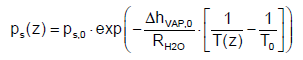 (24)
(24)
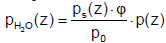
The partial pressure of water vapor can be written as
 (25)
(25)
where ps is the saturated pressure, ΔhVAP,0 is the evaporation enthalpy of water at standard conditions depending on T0, RH2O is the gas constant of water (464 J kg‑1 K‑1) and ϕ is the relative humidity of the atmosphere.
The figure also shows the associated decrease of the partial pressure of water vapor.
 (26)
(26)
Where in the average humidity of the atmosphere is assumed to be ϕ = 80% and the total pressure decreases according to the barometric formula:
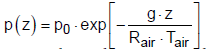 (27)
(27)
where p0 = 1 bar is the pressure at the ground, Rair is the gas constant of air (287 J kg-1 K-1), g is the gravity constant, Tair is the mean temperature of the air and z is the coordinate of the height. The calculated profiles of water vapor concentration and temperature in the atmosphere show acceptable agreement with the actual measured data published in [13,14].
The integration over the height leads to the mean product of partial pressure and beam length.
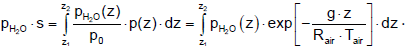 (28)
(28)
For the emissivity below the clouds the product of partial pressure and beam length is integrated from the surface to the height of the clouds zc, which is approximately on average at 3 km. For the emissivity of the cloud-free sky integration to infinity is needed. The value of the integral, the optical thickness, is shown in Figure 6. The final accumulation is reached at a height of about 8 km.

Figure 6: Optical thickness of water vapor in the atmosphere.
To determine the optical thickness of the carbon dioxide, it must be taken into account that the concentration c is constant with the height. When pCO2 = CCO2 · p(z) the optical thickness follows:
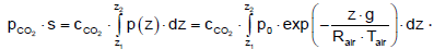 (29)
(29)
The results are shown in Figure 7. The concentration of 355 ppm is used, which was measured in the reference year 1990 for the assessment of CO2 reduction. The optical thickness for the gas between the Earth and the clouds is 0.90 bar⋅m, for a cloud-free sky and space it is 2.72 bar⋅m and for the gas between the clouds and space it is 1.43 bar·m. The final accumulation is reached at a height of about 30 km. Only the radiation behavior below this level influences the Earth’s temperature.
In Table 2, the products of the partial pressure and the beam length of individual gases are presented. For the relevant average temperatures of the atmosphere, values are selected, which belong to the half of the maximum value of the optical thickness. These temperatures are 7°C below the clouds, -55°C above the clouds and -15°C for the cloud-free atmosphere.

Figure 7: Optical thickness of carbon dioxide in the atmosphere.
| Gas i | Pi × s = bar × m | ||
|---|---|---|---|
| below the clouds T = 7°C | above the clouds T = -55°C | cloud-free sky T = -15°C | |
| H2O | 20.69 | 4.04 | 24.97 |
| CO2 | 0.90 | 1.43 | 2.72 |
Table 2: Optical thickness of the individual gases.
The temperature above the clouds is often displayed in airplanes as the outside temperature. As shown in Figure 7, the flying height of 11 km lies approximately in the average range of the optical thickness.
Emissivity of H2O and CO2: With dependence on partial pressure, beam length and temperature, the emissivity of both H2O and CO2 can be found in the figures and diagrams of heat transfer books [10,11]. Using these graphical solutions is the most practical method [1]. But in all heat transfer books the emissivity is only specified above 20°C. Temperatures below 20°C are especially relevant to describe the effect of green house gases in the atmosphere. Therefore, reasonable approximations are necessary.
The emissivity of water vapor is shown in Figure 8. It is obvious, that the emissivity at large values of the product of pressure and beam length, at about more than 5 bar⋅m, is nearly independent of temperature [15-18]. In literature, no emissivities could be found for optical thicknesses above 10 bar⋅m. So, an extrapolation is used to assume the emissivity of water vapor within the relevant region of the atmosphere, as presented in Table 2. Figure 9 shows the emissivity of water vapor as a function of the optical thickness. The approximation used is given within the figure as well. For the relevant values of the atmosphere the graph stays relatively flat.

Figure 8: Emissivity of water vapor [17,18].

Figure 9: Emissivity of water vapor in the atmosphere.
The emissivity of carbon dioxide is shown in Figure 10. The values are taken again from Lallemant et al. [17]. At short-wave radiation and high temperature the emissivity goes to zero because carbon dioxide has no absorption bands less than 2 μm. The largest absorption band of carbon dioxide is in the range of 12 to 18 μm [1]. Only this band is significant for the radiation in the atmosphere. Therefore, the emissivity shows a maximum at a temperature of about 250 K [10,19]. At wavelengths above 18 μm carbon dioxide has no bands, therefore the emissivity goes to zero at temperatures below 70 K and extremely long-wave radiation [9].

Figure 10: Emissivity of carbon dioxide [10,17,19].
It is clearly visible, that, at low temperature, the emissivity not only rises with the concentration, but also with an increase of temperature. The increase of the temperature in the atmosphere results in an increase of the emissivity, even with a constant CO2 concentration.
The emissivity of the carbon dioxide is a function of the optical thickness as shown in Figure 11. The illustration shows that all three emissivities are situated in the flat range of the curve. Obviously, the emissivity would increase if the optical thickness increases further due to an increase of the concentration of carbon dioxide.
All considered gas layers in the atmosphere consist of H2O and CO2. The emissivity of the mixture is given as:

Figure 11: Emissivity of carbon dioxide in the atmosphere.
 (30)
(30)
The gas emissivity does not significantly increase for CO2 concentrations above the current value of about 400 ppm, because the emissivity below the clouds is dominated by H2O.
Determination of heat fluxes
By using the previously given equations, the heat fluxes in the atmosphere due to radiation can be calculated. The mean emissivity of the Earth is 0.95 [15,16]. The average value of the emissivity of the clouds for the entire atmosphere is unknown, so the temperature of the Earth cannot be calculated with the model presented here. The aim of the model is not to calculate the temperature, but to show the effect of increasing CO2 concentrations. Therefore, the model is adjusted to the known surface temperature of the reference year 1990 [1]. The results are shown in Figure 12. To get 15°C as the Earth’s temperature in 1990, the cloud emissivity was adjusted to 0.96. Thus, the average heat flows in the atmosphere and the ambient temperature of the earth surface can be simulated well with the presented model.

Figure 12: Heat fluxes in the atmosphere.
Influence of CO2 Concentration
For the current climate analysis, it is of great interest to know how strongly CO2 influences the climate and to what extent the temperature of the Earth increases with an increase in the CO2 content. The measure of how sensitively the temperature reacts to a change in the carbon dioxide content is called the climate sensitivity. Climate sensitivity is the change of the average global ground level temperature caused by a doubling of the CO2 concentration. It is assumed here that the system is at equilibrium before and after the change. There are several possibilities for the assessment of how the climate system reacts to a doubling of the carbon dioxide concentration.
Based on the previously presented equations, the dependency of the Earth’s surface temperature on the carbon dioxide concentration was calculated. Figure 13 shows how the temperature of the Earth increases with the CO2 concentration. Without CO2, the temperature of the Earth would be 4 K colder. It is shown that, for a doubling of the carbon dioxide concentration from 355 ppm to 710 ppm, the temperature increases from 15°C to 15.43°C. Therefore the climate sensitivity for this model is 0.43°C.

Figure 13: Increase of Earth temperature with CO2 concentration.
In the present model, global mean parameters are used as constants, e.g. cloud height, relative humidity and Earth emissivity. Table 3 shows that the effect of doubling of CO2 is hardly influenced by them. So, the precision of the previously assumed model constants does not affect the dependency between CO2 concentration and earth temperature much.
| Model constant | Variation | Climate Sensitivity |
|---|---|---|
| Cloud height | 2000 m | 0.42 K |
| 4000 m | 0.43 K | |
| Relative humidity | 70% | 0.43 K |
| 90% | 0.42 K | |
| Earth emissivity | 0.97 | 0.43 K |
| 0.93 | 0.43 K |
Table 3: Model sensitivity.
Furthermore, it is possible to analyze the climate in the past. How did the system react to a change in the carbon dioxide concentration? Using the measured data and the state of knowledge of past climate fluctuations, the influence of CO2 concentration on the climate during a certain period of time can be calculated. The reasons for the historical increase in temperature are various. The effect of CO2 and H2O play an important role, but there are side effects, other greenhouse gases e.g. methane and further reasons not discussed here. Between the beginning of the industrial revolution in 1860 and 1990 the global warming was 1 K. CO2 contributed only 0.2 K as Figure 13 shows. This additional temperature increase is traced back to side effects, so that a future temperature increase is also forecasted which is higher than the calculated 0.43 K.
As a side effect, it is taken into account that the water vapor concentration in the atmosphere increases because of the CO2 caused temperature increase. This leads to an increase of the emissivity of vapor and interferes with the back radiation from the Earth’s surface. The increase of water vapor in the atmosphere leads to more cloud forming, which also should affect the temperature increase. The different parameters affect the temperature on the Earth very sensitively. Therefore, the different global climate models produce different results because of the influences of side effects. Thus, the predicted temperature increases are in the range of 0.5 to 5 K [1]. The temperature increase calculated with the simple model presented in this paper lies in the lower range.
Conclusions
With a one dimensional mathematical model, the mechanism of global warming is explained. The fundamental physical principles generally used in the engineering field are used to calculate the heat fluxes due to radiation with an atmosphere containing CO2 and H2O.
With an increasing gas emissivity because of an increasing CO2 concentration the overall emissivities decrease. Therewith, the CO2 acts as a radiation shield for the radiation from the Earth surface. This increasing resistance for the radiative heat flux must be compensated with an increasing Earth temperature.
When the CO2 concentration is doubled, the temperature of the Earth increases by 0.43 K. Since 1860, the Earth’s temperature has already risen due to anthropogenic CO2 emissions by 0.2 Kelvin. The measured increase of about 0.9 Kelvin is attributed to side effects caused by the CO2 related temperature increase. Therefore, a temperature increase of more than 0.43 Kelvin is predicted for the future.
References
- Specht E,RedemannT,Lorenz N (2016) Simplified mathematical model for calculating global warmingthrough anthropogenic CO2.Int J ThermSci102: 1-8.
- Foong SK(2006) An accurate analytical solution of a zero-dimensional greenhousemodelfor global warming.Eur J Phys27: 933-942.
- Knox RS(1999) Physical aspects of the greenhouse effect and global warming. Am J Phys67:1227-1238.
- Barker JR, RossMH (1999) An introduction to global warming. Am J Phys67: 1216-1226.
- http://www.esrl.noaa.gov/about/staff.html
- Kiehl JT,Trenberth KE (1997) Earth's annual global meanenergy budget. B Am MeteorolSoc 78: 197-208.
- Wang WC,Rossow WB,Yao MS,Wolfson M (1981) Climate sensitivityof a one-dimensional radiative-convective model with cloud feedback. J AtmosSci38:1167-1178.
- Liou KN (2002) Anintroduction to atmospheric radiation
- ModestMF (1993) Radiative heat transfer, McGraw-Hill series in mechanical engineering.Heat Transmission Heat Radiation and absorption, New York: Mcgraw-Hill, pp: 832.
- Specht E (2014) Heat and mass transfer in thermal processengineering, VulkanVerlag Essen,German.
- Mills AF (1999) Basicheat and mass transfer, Prentice Hall, Upper Saddle River, New Jersey.
- Kondratyev KY(1969) Radiation in the atmosphere. IntGeophysSeries12: 124-129.
- Kunz A,Muller R, Homonnai V, Jánosi M, Hurst D, et al. (2013)Extending water vaportrend observations over Boulder into troppause region: Trend uncertainties andresulting radiative forcing. J Geophys Res-Atmos118: 11,269-11,284.
- MastenbrookHJ (1968) Water vapor distribution in the stratosphere and high troposphere. JAtmosSci25: 299-311.
- RoedelW (1992) Physicsof theenvironment. Theatmosphere,Springer Publisher, Berlin, Heidelberg, NewYork, Germany.
- Weischet W,Endlicher W (2008) Introduction tothegeneralclimatology, Gebrüder Borntraeger Verlagsbuchhandlung,Stuttgart, Germany.
- Lallemant N, SayreA,Weber R (1996) Evaluation of emissivity correlations for H2O-CO2-N2/airmixtures and coupling with solution methods of the radiative transfer equation.ProgEnergy CombustSci22: 543-574.
- (1994) TheCRC Handbook of Mechanical Engineering (2ndedn.). In: Kreith F,Goswami Y (eds) CRC Press, Boca Raton, FL.
- LorenzN (2012) Simplified one-dimensional model for calculating global warmingthrough anthropogenic CO2, dissertation. Otto von GuerickeUniversity Magdeburg(in German).
Relevant Topics
- Aquatic Ecosystems
- Biodiversity
- Conservation Biology
- Coral Reef Ecology
- Distribution Aggregation
- Ecology and Migration of Animal
- Ecosystem Service
- Ecosystem-Level Measuring
- Endangered Species
- Environmental Tourism
- Forest Biome
- Lake Circulation
- Leaf Morphology
- Marine Conservation
- Marine Ecosystems
- Phytoplankton Abundance
- Population Dyanamics
- Semiarid Ecosystem Soil Properties
- Spatial Distribution
- Species Composition
- Species Rarity
- Sustainability Dynamics
- Sustainable Forest Management
- Tropical Aquaculture
- Tropical Ecosystems
Recommended Journals
Article Tools
Article Usage
- Total views: 14885
- [From(publication date):
specialissue-2016 - Apr 02, 2025] - Breakdown by view type
- HTML page views : 13823
- PDF downloads : 1062