Analysing Relationship between Air Pollutants and Meteorological Parameters Using TRA, PCA & CA: A Concise Review
Received: 03-Mar-2023 / Manuscript No. EPCC-23-90721 / Editor assigned: 06-Mar-2023 / PreQC No. EPCC-23-90721 (PQ) / Reviewed: 20-Mar-2023 / QC No. EPCC-23-90721 / Revised: 21-Mar-2023 / Manuscript No. EPCC-23-90721 (R) / Published Date: 28-Mar-2023 DOI: 10.4172/2573-458X.1000327
Abstract
Air pollution plays a significant role in causing respiratory illnesses and fatalities, and it also contributes to global warming and environmental degradation. Recent advances in remote sensing technology have improved our understanding of the complex interactions involved. This review study offers a comprehensive examination of the current understanding of air pollution, highlighting areas where analytical and detection methods have been improved.The study highlights recent studies that use a worldwide monitoring system with established procedures to keep an eye on new environmental concerns. The study also evaluates the efficiency of different correlation methods, like TRA, PCA, and CA, in analysing the association among meteorological parameters and air pollution, and suggests the most appropriate techniques for the analysis.
Keywords
Air Pollution; Atmosphere; Space-borne instrument; PCA; CA; Air Mass; Trajectory Regression Analysis; Meteorological Variables; IASI (Infrared Atmospheric Sounding Interferometer, TROPOMI (Tropical Atmospheric Monitoring Instrument; ESA (European Space Agency); NOAA-ARL (National Oceanic and Atmospheric Administration’s Air Resources Laboratory)
Introduction
As per the WHO, air pollution has become the prime reason for mortality, with projections estimating that it will impact 6.5 million people by 2050. The implications of air pollution on public health varies, also it is not equally distributed globally, with Asia experiencing the highest levels. The average adult inhales 10 liters of air per minute, and this amount increases during physical activity. Children, elderly people, and individuals with respiratory or cardiovascular conditions are at an increased chance of being harmfully influenced by air pollution. The Health Effect Institute’s research shows that air pollution plays a substantial role in causing deaths and a significant reduction in the number of healthy years of life. It also causes 7.6% of all deaths, with respiratory and cardiovascular diseases being the main contributors. In Europe alone, air pollution leads to an additional 800,000 deaths each year (Figure 1).

Figure 1: Share of deaths attributed to outdoor air pollution, 2019 [23].
The figure illustrates the yearly average mortality rate caused by PM2.5 and ozone in a 100 x 100 km area, using a range of colors. In the map, areas with lower concentrations of air pollution are represented by white color, suggests that they are not a major hazard to human health. Alternatively, regions with a more profound coloration signify the presence of elevated amounts of harmful pollutants, which can be deleterious to the well-being of individuals.
Air pollution is not only limited to its effects on visibility, as citizens can easily observe, but it can also impact other aspects of the atmosphere. One significant effect is on the formation of precipitation, which can lead to changes in weather patterns. By studying the impact of pollutants on these atmospheric mechanisms, researchers can gain a better understanding of how pollution affects weather in a specific region. Furthermore, air pollution is connected to alterations in the occurrence and timespan of fog, particularly in urban areas.
Air pollutants have the potential to affect the surrounding temperature by absorbing radiant energy. While the potential effects of increased carbon dioxide concentrations on the environment have been widely publicized, other factors such as nitrogen dioxide and aerosols may also contribute to pollution in local urban areas. Remote sensing is commonly used for environmental studies, including the monitoring of water and air standards. It is important to mention that the Earth’s atmosphere can impact satellite imagery of the planet’s surface by altering the solar spectrum. As a result, the signal captured by the sensor of satellite’s, encompasses the impact of atmosphere and the Earth’s surface. Measuring changes in radiation due to the impact of tropospheric aerosols is difficult because of the diverse nature of aerosols in terms of their types, times, sizes, and locations [1]. To retrieve atmospheric components from remote sensing data, surface reflectance is critical. The signal measured by remote sensors can be impacted by optical atmospheric effects in two manners: geometrically and radiometrically. This means that the signal’s strength can be changed through processes such as diffusion or absorption and its direction can be altered through refraction [2].
The harmful effects of atmospheric pollution, particularly aerosols, have been the focus of recent scientific research. Measuring the visiblerange optical depth of aerosols is a viable approach to approximating the amount of pollutants present in urban areas. Air pollution, a longstanding problem in industrialized and developing countries in the West, is now becoming a growing concern in East Asian developing countries. The absence of information about the characteristics of pollutants is a major challenge in assessing their impact on the climate.Analysing pollutants which are available in our atmosphere is itself a complex task. An adverse health effects associated with small particles have brought attention to the air pollution problems, which is a notable environmental problem that predominantly impacts urban areas. The review study’s aims are stated as follows:
• To examine studies that utilizes TRA to find the sources of PM pollutants.
• To analyze studies that employ clustering techniques to recognize the relationship among air pollutants and meteorological factors.
• To evaluate research studies that implement PCA to investigate the correlations among meteorological factors, air pollutants, or both.
• To document the process of bibliographic research.
The framework of this review study is categorised as: Section 1. concentrates on air pollution, highlighting the significant pollutants and how they have changed over time. Section 2 focuses on literature review of related research studies published in recent years. Section 3. summarizes the methodology adopted for this research review, Section 5. Represents the result of the searches in brief manner. Section 6. Includes to conclude the research review.
Related Studies (Table 1)
| Citation | Research Area | Publication Year | Conclusions |
|---|---|---|---|
| [26] | North Chennai-India | 2013 |
|
| [15] | China | 2014 | The levels of pollutants (CO, SO2 & PM10/PM2.5) detected at higher level during the winter season than in the summer. |
| [21] | Beijing, Shanghai, and Guangzhou- China | 2015 | The study found that during the winter season, there was a correlation between NO2, SO2, CO, and PM concentrations with both wind speed (WS) and ozone (O3) levels. Additionally, these pollutants were also correlated with temperature. |
| [38] | China | 2017 | A declining pattern was observed in the yearly averages over a three-year span. However, the peak levels persisted to occur during the winter and the down trend during summer. |
| [41] | Tehran- Iran | 2018 | The research discovered significant decline in PM2.5 and O3 levels over the course of conducted study. PM2.5 concentrations were observed at highest level in summer & winter, while the highest O3 levels were detected in spring and summer. |
| [39] | China | 2019 |
|
| [45] | Tabriz- Iran | 2020 |
|
| [14] | China | 2020 | The levels of PM10, CO, SO2 & PM2.5 declined by 13.5%, 22.1%, 21.5%, and 46.4%, respectively. However, the decrease in NO2 was less clear at 6.3%. On the other hand, O3 concentration significantly increased by 13.7%. |
| [33] | China | 2020 | The average annual levels of PM10, SO2, CO, and PM2.5 indicated a declined movement, while NO2 and O3 density showed an upward trend. Additionally, the deepest levels of these pollutants were reported during the summer season, while the maximum levels were observed in winter season. |
| [03] | Saudi Arabia | 2021 | In Italy, cities with stronger wind velocities have fewer COVID-19 cases. |
| [49] | West USA | 2006 | Waterborne Transport was identified as one of the key contributors of PM (particulate matter) pollution. |
| [24] | Arctic | 2010 | Russia was found to be the primary source of 67% of the observed black carbon concentration. |
| [7] | Athens | 2013 | As per the findings, more than 40% of the PM (particulate matter) pollution in Athens was found to originate from areas that are located more than 500 km away. |
| [8] | Arkansas | 2013 | Effect of combustion on PM (PM <2.5mm) concentrations was harmful for human health. |
| [28] | Birmingham, Amsterdam, Helsinki and Athens | 2013 |
|
| [9] | Paris | 2014 | It has been shown that approximately 50% of the air mass contributing to PM10 (<10 mm) concentrations comes from local sources. |
| [40] | Doña Ana County | 2014 | Sources inside a 500 km range were found to contribute to increased PM (particulate matter) concentrations. Road dust was established as one of the primary contributors to PM2.5 and PM10, which are particulate matter less than 10 mm and 2.5 mm in size, respectively. |
| [11] | Marseille | 2018 | The local emissions, such as those from traffic and heating, have contributed to increased PM (particulate matter) concentrations. The combustion of fuels in these local sources were recognized as a major source of Particular Matter emissions. |
Table 1: Literature review for related studies.
Air Pollution
Pollutants & Trends
Pollutants are a mixture of different chemicals that can have negative effects on public health, unlike greenhouse gases that impact the climate. These contaminants may be released directly from their sources or generated through chemical reactions in the atmosphere. The size, shape, & chemical structure of these gases and elements can affect environment and various living organisms. Assessing the specific health consequences of individual pollutants is complex, however, recent studies have formed a association among air particle concentrations and health outcomes. It has been known for some time that countries with high levels of pollution have lower life expectancy rates [2].
Air quality guidelines usually specify and set criteria for several air pollutants like PM10 & PM2.5 (Diameter <10 mm), CO, NH3, O3, NO2 and SO2. These sources of pollution arise from a variety of human activities, including transportation, heating, industry, and agriculture, among others, as indicated in Table 2.
| Pollutant | Source | Environmental and Health Effects |
|---|---|---|
| Sulfur dioxide (SO2) | Fossil fuels Burning, including oil, coal, & gas, in power plants, industries, automobiles, planes, and ships. | The respiratory system can be impacted, and the eyes may experience irritation. |
| Nitrogen dioxide (NO2) | Fossil fuels in industrial and traffic sources | Can lead to respiratory issues and is linked to early death. |
| Carbon monoxide (CO) | Inadequate fuels burning (carbon), such as natural gas, gasoline, coal ,oil, and timber. | Include headaches, tiredness, dizziness, drowsiness, and nausea. Chest pain may also occur in individuals with angina. |
| Ozone (O3) | The process of converting carbon monoxide, methane, or other volatile organic compounds into different forms through interaction with nitrogen oxides and exposure to sunlight. | Asthma, decreased lung capacity, and various respiratory illnesses. |
| Ammonia (NH3) | Nitrogen fertilizers and livestock manure. | Causing harm to the environment through processes like acidification and over-fertilization. |
| Particulate matter (PM) | Traffic and industry activities for example energy production, mining, building, and the cement production. | The presence of air pollutants poses a notable risk to the well-being of the general population as they can infiltrate the respiratory system and travel through the bloodstream. |
Table 2: Major atmospheric pollutants with sources and effects.
Pollutant emissions vary in different countries, and the regulation of air quality varies accordingly. About 50 countries currently regulate air quality, with different thresholds for population warnings. Figure 2 shows the changes in emissions of major pollutants from 2010 to 2020. In most industrialized countries where coal is no longer used, ozone, ammonia, and PM2.5/PM10 were the most frequently occurring pollutants that exceed harmful thresholds. Ammonia, which is linked to livestock and fertilizers, is particularly hard to supervise.

Figure 2: Trends in Air Emissions of Selected Pollutants 2010-2020 [28].
China and India are recognized as the countries with the highest levels of pollution. India has started taking measures to control air pollution, including efforts to reduce domestic emissions. Despite the fact that air quality in Asia remains a concern, significant improvements have been observed in recent years (as shown in Figure 3), indicating that air quality management efforts seen a rapid and vital consequences on air standards not only in Asia but also globally.

Figure 3: Global Energy-related CO2 Emissions by Region 1965-2021.
Over the past few decades, remote sensing techniques for monitoring atmospheric gas concentrations have greatly improved and can now accurately assess air quality. Atmospheric composition is commonly analyzed using spectrometers with a wide range of spectral resolutions, from thermal infrared to ultraviolet. The use of a blend of ground-based measurements, atmospheric models, and spatial observations from satellites is critical in many atmospheric applications and research articles, Assisting in the expansion of our knowledge of physical and chemical processes on both a local and global level. Initially, worldwide space observations of gases were mainly devoted to measuring ozone and water vapor during 1980s. However, with improvements in measurement techniques and species concentration search algorithms. Thanks to technological advancements, it is now feasible to gain more accurate information about various gas concentrations and trace pollutants, including those on a regional or local level, with enhanced vertical precision. This means that it is now possible to gather quantitative information about certain reactive substances at the Earth’s surface with a higher level of accuracy.
Passive satellite remote sensing technology can be employed to assess the atmospheric spectrum by examining the interplay between radiation, including sources such as radiation emitted by the Earth or atmosphere, atmospheric molecules, and sunlight. By analysing the spectral signatures of different molecules, the concentration of these molecules can be determined at different altitudes or within a vertical column. Each spectral signature has a distinct characteristic that identifies the molecule and its concentration. To accurately determine the atmospheric densities from raw satellite spectra, it is necessary to have additional information, such as details about the instrument used, spectral data, and atmospheric conditions.
Currently, there exist several satellite instruments that can measure air pollution. IASI [3] and TROPOMI [4] are two modern instruments that utilize visible UV and thermal infrared radiation, respectively.
These instruments have proven their ability to precisely measure the amount and variation of major air pollutants. TROPOMI is a multispectral imaging spectrometer that operates in visible, ultraviolet, near-infrared, and infrared spectral bands (Table 3). Launched in October 2017 by the ESA, TROPOMI provides precise and highresolution space-based monitoring of pollutants like ozone, nitrogen dioxide, sulfur dioxide and formaldehyde (HCHO), which was not previously possible with a resolution of 3.5 × 7 km2.
| Sr. No | Optical Channel | Performance Range(nm) | Spectral Sampling (nm)/oversampling | Spectral Range (nm) | Products |
|---|---|---|---|---|---|
| 1 | VIS | 370-490 | 0.18/4 | 360-495 | O2-O2 Cloud Fraction/Pressure; NO2 |
| 2 | NIR | 710-775 | 0.12/4 | 710-775 | Cloud optical Pressure /thickness/ /Fraction; H2O, Aerosol height distribution. |
| 3 | SWIR | 2305-2385 | 0.125/2 | 2305-2385 | CH4, CO, |
| 4 | UV1 | 270-310 | 0.27/4 | 270-320 | O3 |
| 5 | UV2 | 310-370 | 0.12/4 | 295-380 | SO2 , O3, HCHO |
Table 3: TROPOMI and heritage instruments spectral ranges.
The IASI instrument, developed by CNES and EUMETSAT, is capable of measuring pollutant levels in the thermal infrared spectrum through 8,641 channels. Its spectrum allows for the detection of over 31 different molecules. Three identical IASI devices were launched on Metop-C (Nov 7, 2018), Metop-B (Sep 17, 2012), and Metop-A (Oct 19, 2006). The data collected by these devices is analyzed and processed in next few years, enabling the creation of a global map of gas concentrations within three hours of measurement (Figure 4).

Figure 4: IASI Spectrum with Highlighted Ranges for Temperature, Water Vapor, and Ozone Profile Inversion in Units of Brightness Temperature.
The combination of cross-platform, satellite, and on-site measurements offers a more comprehensive understanding of the atmosphere’s chemical composition. In situ measurements provide greater accuracy at a local level, while satellite measurements offer wider coverage and information on the movement of pollution clusters. These satellite observations play a crucial role in limiting emissions, validating our understanding of atmospheric processes, and improving peak pollution predictions. The infrared and ultraviolet observations obtained from these devices provide valuable information for studying pollution globally. The Copernicus Atmospheric Composition Monitoring System (CAMS) combines data from multiple satellite instruments to create regional and global models, providing practical information on air quality and key pollutants.
Methodology
The review study conducted a comprehensive literature search in various databases, including PubMed, Web of Science, Scopus, SciELO, and ScienceDirect, using keywords such as particles, regression analysis, air mass trajectory, principal component analysis, cluster analysis, and meteorological variables. The synonyms of the search terms were merged by using either “AND” or “OR” operators, depending on the requirements of each database. For the first objective, the focus was on regression analysis to examine the connection among air pollutant concentration and total residence time of air masses in a designated area. To expand the search, other statistical methods such as generalized linear models were also considered. The focus of the study is to utilize Total Residence Time Analysis (TRA) to analyze air pollutant concentrations based on the duration air masses remain in a particular area (as described in research study conducted by Rodopoulou [5]; Xu [6]; and Kassomenos and Dimitriou [7]. To achieve the second and third objectives, a search was conducted using terms related to principal component analysis, cluster techniques, meteorological factors, and particulate matter (Figures 5 and 6).

Figure 5: Prisma Diagram for Objective 1.

Figure 6: Prisma Diagram for objective 2 & 3.
For the first objective (TRA), the authors considered publications from 2006 to 2021, while for the second objective (CA) and the third objective (PCA), limited to 2011-2021. The reason for this variance is because of vast recent publications studies in these areas. It should be noted that between 2011 and 2021, there were 537 studies listed in Science Direct alone on CA and PCA, while there were 296 studies listed on the trajectories of particles in air masses and pollutants.
The selection criteria inherited for the exclusion and inclusion of studies are as follows:
• Time frame:
Objective 1: Articles published before 2006 were excluded.
Objectives 2 and 3: Articles published before 2011 were excluded.
• Analysis type:
The literature must use multivariate statistical models, with a preference for regression models,
general linear models, CA (Cluster Analysis), or PCA (Principal Component Analysis).
• Purpose of analysis:
Objective 1: To determine the relationship between specific contaminants (air pollution) and air mass trajectories.
Objective 2: To collection locations or time frames with same behavior.
Objective 3: To find the correlation among meteorological variables and air pollutants.
Results
This section is organized based on the objectives of the study. The subsection “Orbital Regression Analysis” covers articles associated to Objective 1 (TRA), while the subcategory “CA & PCA” covers articles related to Objectives 2 (CA) and 3 (PCA).
Orbital Regression Analysis:
A preliminary search for Objective 1 resulted in 712 articles, of which 15 were selected after the filtering process (Figure 3). These selected papers study the trajectories of particles in the air mass and were found in databases such as ScienceDirect, Web of Science, and PubMed, wasn’t found articles in SciELO database (Figure 3). All included papers used trajectory regression analysis (TRA), which is also referred to as multiple regression analysis, TrMB model (Track Volume Balance) or regression analysis. The dependent variable in these investigations is the level of atmospheric pollutants, whereas the independent variable is the duration of air masses spent in a designated region. The amount of independent variables is determined by the number of areas established based on geographical similarities and proximity to the receptor location. This approach is described in various works such as [9-12].
CA and PCA
The number of articles found under Objectives 2 and 3 and the selection criteria used for these objectives are not specified in the text. The initial search for Objectives two and three provided 1843 articles, from them 25 were selected after applying filtering steps. These selected articles apply Principal Component Analysis and Cluster Analysis to cluster locations / timespans with correlation between atmospheric pollutants and meteorological variables. Out of the twenty-five articles, ten used PCA, six articles used CA, and nine articles used both CA and PCA. The search in the SciELO database did not yield any relevant results.
Of the 11 articles using CA, 5 grouped monitoring stations or locations, two grouped air pollutants, and 4 grouped meteorological variables. Some studies grouped dates or day hours. Eight of the nineteen studies that utilized PCA included both meteorological variables and air pollutants in their main components, while the other eleven studies only focused on the air pollutants. One study related locations, and another related meteorological variable.
Discussion
In this section, the most significant papers relevant to Objectives one (discussed in “Trajectory Regression Analysis” sub-section) and Objectives two and three (discussed in “Cluster Analysis & Principal Component Analysis” sub-section) will be discussed.
Trajectory Regression Analysis (TRA)
This model formulated as Eq 1 [13]:
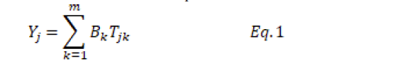
The approach of the Trajectory Regression Analysis (TRA) entails evaluating the relationship between the duration of air masses spent in a particular region and the corresponding levels of air pollution. This duration is determined by aggregating the quantity of trajectory points found within a defined area. The impact of each region on the pollutant concentration is being evaluated (PMj) is established by multiplying the contribution factor (Bk) and the total residence time (Tjk).
The input for TRA is the particle trajectory, which can be obtained using the HYSPLIT model created by NOAA-ARL. This model, utilized in various studies such as those conducted by Dimitriou and Kassomenos [14,15], Xu et al. [16], Chalbot et al. [17], Kavouras et al.,[18] and Huang et al. [19,20] has been widely used for regression analysis. The HYSPLIT model calculates the backward path of air masses reaching the research area using meteorological parameters.
The HYSPLIT model can utilize different sources of meteorological data to determine backward air mass trajectories. Some research studies, represented by Kavouras et al. [21]and Chalbot et al. [22,23], use the Global Data Assimilation System (GDAS), while others, like Huang et al. [24], use the NCEP/NCAR global reanalysis data. Other studies, such as those by Xu [25] and [26], utilize the Eta Data Assimilation System (EDAS). However, exact meteorological dataset used by Dimitriou and Kassomenos [27,28] is not specified in their research.
The air mass trajectory calculations in the reviewed studies aimed to reach a receptor site at 500 meters above earth’s surface. The calculation considered the average boundary layer heights for climatological purposes, with the goal of assessing the impact of varying atmospheric circulation patterns. To compute the trajectories using the HYSPLIT model, it was necessary to define the duration in terms of the number of days and hours for which the calculation was to be performed. For instance, Xu et al. [29] utilized 8 back trajectories per day for a period of 8 days and 24 hr/day, resulting in a total of 1536 trajectory points/day. Meanwhile, the quantity of backward air mass trajectories employed in various studies varied. Huang et al. [30] computed 12 back trajectories per day for a 10-day span, whereas Chalbot et al. [31], Kavouras et al. [32] and Chalbot et al. [33] calculated 24 back trajectories per day for a 5-day period [34]) computed 6 back trajectories per day for a 5-day span, and Kassomenos and Dimitriou [35,36] calculated 24 back trajectories per day for a period of 3 days.
To understand the effect of different regions on air pollutant concentrations, various studies have applied the Total Residence Time Analysis (TRA) method. The primary objective of these investigations was to ascertain the impact of air masses originating from different locations on the daily levels of PM10 and PM2.5, and to pinpoint the sources of PM emissions. The results showed that local sources can play a significant role in air pollutant concentrations. For instance, a study by Dimitriou and Kassomenos [37] in Paris, it was discovered that nearly 50% of the daily PM concentration could be attributed to sources within the local vicinity. Another study by Kavouras et al. [38] in four cities showed that central Europe was the primary contributor to air pollutants in Amsterdam and Birmingham, while northern Africa and the Mediterranean Sea were the main contributors to Athens. In the United States, the Trajectory Regression Analysis (TRA) model was employed to assess both the regional and local aspects of ammonium sulfate , ozone, and PM levels, it was found that emissions from shipping and ports along the Pacific Coast had a predominant influence on the levels of ammonium sulfate concentration in the Western United States [39]. These studies emphasize the significance of taking into account both local and regional sources when assessing air pollutant levels.
The TRA method has been used in the reviewed studies to explore the impact of air masses originating from specific geographic areas on air pollutants densities. The aim is to determine the extent to which various geographical regions are responsible for the daily densities of PM2.5 and PM10. For example, Dimitriou and Kassomenos [40] applied the TRA method in a study in Marseille, France, to assess the contributions of PM10 and PM2.5 from 15 regions during different seasons, and they introduced a novel predictor variable to evaluate the impact of atmospheric spread.
The Trajectory Regression Analysis (TRA) is a valuable approach for identifying the sources of PM emissions and calculating the impact of specific regions on atmospheric pollutant levels. This assumption is made in the models used in the studies, which expect that the pollutant concentration data follows a normal distribution and can have any real value, resultants values predicted to be a positive as data only deals with pollutant concentrations. However, this assumption of independence may need to be re-evaluated in light of the fact that the used data is organised in a temporal manner. Further studies could integrate TRA with time series models or incorporate additional variables, like meteorological data, to enhance the accuracy of determining daily PM contribution of study area.
Cluster Analysis (CA) and/or Principal Component Analysis (PCA)
The papers analyzed in reviewed studies use either CA or PCA, or a combination of both, as multivariate techniques to uncover complex relationships among variables. While CA groups observations together without making assumptions about their quantity or structure, The primary goal of PCA is to recognize a limited number of linearly uncorrelated combinations of the real variables, which are referred to as principal components. The application of these techniques is widespread in various research studies and holds a critical function in determining the spatial attributes of contaminant patterns, as well as pinpointing the origins of pollutants.
Studies using Cluster analysis
In four studies, Cluster Analysis (CA) was used to explore relationships between variables. Two of these studies grouped monitoring stations, as seen in [41] and [42], while the other two studies grouped days of the year, as in [43] and [44]. The grouping of days was aimed at identifying similar meteorological conditions [45] or air pollutant profiles [46], while the monitoring stations were grouped together in order to classify areas that show similar patterns in air pollutant concentrations [47,48].
In addition, two studies used PCA to uncover relationships between variables. Chen et al. [49] PCA was employed to detect the principal contributors of PM2.5 in a rural region situated in China (northeastern). The results indicated that the most substantial sources of the pollutant were coal combustion, soil dust, and secondary aerosols. Meanwhile, Li et al. [50] used PCA to scrutinize the inceptions of PM2.5 and PM10 in Beijing. The investigation revealed that construction dust and vehicle emissions were the primary sources of PM10, while vehicle emissions, dust storms and coal combustion, were major contributors of PM2.5. These studies demonstrate the usefulness of PCA in source apportionment and highlight the need for effective control measures to reduce PM emissions.
Studies using Principal Component Analysis
A number of the studies that were reviewed implemented PCA to explore the correlations between multiple factors, such as air pollutants and meteorological factors, either independently or in tandem. The aim of using PCA in these studies was to identify the primary sources affecting air pollutant concentration and to assess the combined influence of air pollutants. Moreover, relationship between meteorological factors and air pollutants studied using PCA. In some instances, PCA was paired through regression analysis [51,52].
For instance, Kwon et al. applied PCA to study the impact of climate variables over PM in six subway stations, Seoul and found that PM concentrations were influenced by ventilation inside and outside trains. Meanwhile, Luna et al. [32] applied PCA for analysing the correlation among atmospheric pollutants and meteorological parameters in three climate observation stations of Rio de Janeiro, Brazil, revealing that NO, NOx, and solar radiation had a substantial effect on ozone concentration.
In Hong Kong, He and Lu [23] used PCA to analyze the impact of climate variables on ozone density and assessed those meteorological variables played a role in 31-34% of the ozone variability at two air quality monitoring stations. Schmeling and Binaku [4] in Chicago, PCA was applied to examine the association among climate variables as well as air pollution. During the study conducted in Bogotá, Colombia, it was observed that the four primary components accounted for approximately 70% of the data., Franceschi et al. [17] utilized the outputs from PCA as inputs for artificial neural network models. The PCA revealed a positive association among PM10 density and the meridional component of wind, and a negative connection between PM10 concentration and temperature & wind speed. Conversely, PM2.5 density had a positive relationship with wind direction and relative humidity.
Studies using Principal Component Analysis and Cluster Analysis
In seven studies, PCA and CA were utilized in tandem to enhance the comprehension of the link of pollutants and climate conditions [47,16]. In these studies, utilization of CA was adopted to group observation stations and uncover the spatial trends in air pollution, whereas PCA was employed to recognize the key air pollution provenances. By combining both techniques, the studies aimed to analyze daily air quality patterns and evaluate the most impactful pollutants [22,30].
In Hong Kong, Lu et al. [31] evaluated the use of PCA and CA in determining city areas with same air pollution patterns. They observed that vehicle emissions and wind direction were the primary factors affecting the level of pollutants and determined that both techniques were effective in handling air quality monitoring systems. In Malaysia, Dominick et al. [12] utilized a fusion of multiple regression analysis, PCA, and CA to perform an air quality evaluation. The main sources of pollution were found to be industries, vehicles, and densely populated regions, with PM10 being the most significant contributor to air pollution. The study also discovered that meteorological parameters like wind speed, temperature, humidity and influenced PM10 density levels.
Jassim et al. [27] utilized PCA and CA in Bahrain to categorize observational stations and determine the major reason of air pollution. The observations of study indicate the factors such as power plants, airport and industrial activities, vehicle emissions, and dust storms were significant origins of air pollution. The study also found that wind speed and temperature were positively correlated with air pollutants, while relative humidity was negatively correlated. In Malaysia, Latif et al. [30] combined PCA and CA to study connection among meteorological factors and air pollution. The use of CA and PCA was combined in article presented by Dominick et al. [12] in Malaysia to assess air quality. CA was employed to investigate the daily fluctuations of atmospheric pollutants, while PCA was utilized to recognize the most influential climate parameters.
In Langkawi Island, Halim et al. [22] utilized CA to categorize hours of the day into three groups based on air quality variables, and then employed PCR to examine the effect of climate factors on pollutants. The investigation revealed that humidity, temperature, and wind speed were influential factors in about 93% of Langkawi Island’s air quality, with relative humidity having a negative impact and wind speed and temperature having a positive impact on air pollutants. In Lanzhou, China, Filonchyk and Yan [16] combined PCA and CA to explore the association among climate parameters and pollutants. The results showed consistency, with the 1st PC being attributed to industrial sources and transportation emissions, and the 2nd and 3rd PCs being made up of temperature, relative humidity and visibility respectively. In Rio de Janeiro, Brazil, Ventura et al. [47] utilized PCA and CA to study the correlation among meteorological factors and PM2.5. Their findings revealed that PM2.5 density was not affected by season alteration, and they observed a strong association among PM2.5 density and wind speed. Additionally, studies that utilized both CA and PCA, there are also studies that used one of the techniques exclusively. In Southwestern China, Niu et al. [35] applied CA to categorize the chemical components of rainwater in the Yulong Snow Mountain region. Meanwhile, in a separate study, Zhao et al. [50] utilized PCA to examine the connections between the chemical components of rainwater. Additionally, Martins et al. [34] employed PCA to analyse the relationships between the chemical components of rainwater in Limeira, Brazil. These studies illustrate the versatility of both CA and PCA in various applications. However, the combined use of both techniques, as demonstrated in the study by Dominick et al. [12], offers a more comprehensive analysis of the relationship between variables.
Conclusion
The technique of TRA is widely recognized for identifying the sources of air pollutants, but there is room for improvement in the current models. By incorporating time series data or advanced models, a clearer picture of the behavior of pollutants can be obtained. Although TRA is primarily used for PM, it can also be applied to other pollutants such as carbon black, ozone, and ammonium sulfate. More research is needed in regions outside of Europe, the US, and the Arctic, such as Latin America, Africa, and Asia.
CA and PCA are more commonly used techniques and have been applied in various ways in previous studies. This literature review aims to scrutinize and analyze a wide range of research studies that investigate the connection among meteorological parameters and pollutants. By combining TRA, CA, and PCA, a more comprehensive recognizing of the correlation between meteorological variables, emission sources and air pollutants can be obtained. Using TRA to determine emission sources, CA to group cities based on weather patterns and pollutant behavior, and PCA to quantify the relationships between variables, a spatial model between cities can be created. This review is a novel examination of studies that employs PRISMA guidelines in the analysis of meteorological variables and air pollutants, utilizing CA, PCA and TRA.
References
- Austin E, Coull B, Thomas D, Koutrakis P (2012) A framework for identifying distinct multipollutant profiles in air pollution data. Environ Int 45: 112-121.
- Brunekreef B (1997) Air pollution and life expectancy: is there a relation? Occup Environ Med 54: 781-784.
- Ben Maatoug A, Triki MB, Fazel H (2021) How do air pollution and meteorological parameters contribute to the spread of COVID-19 in Saudi Arabia? Environ Sci Pollut Res Int 28: 44132-44139.
- Binaku, Katrina, Schmeling, Martina (2017) Multivariate statistical analyses of air pollutants and meteorology in Chicago during summers 2010-2012. Air Quality, Atmosphere & Health 10: 1-10.
- Clerbaux C, Boynard A, Clarisse L, George M, Hadji-Lazaro J, et al.(2009) Monitoring of atmospheric composition using the thermal infrared IASI/MetOp sounder. Atmos Chem Phys 9: 6041–6054.
- CETESB (2016) Companhia Ambiental do Estado de São Paulo.
- Kavouras GI, Chalbot MC, Lianou M, Kotronarou A , Christina Vei I (2013) Spatial attribution of sulfate and dust aerosol sources in an urban area using receptor modeling coupled with Lagrangian trajectories. Pollution Research 4: 346-353.
- Chalbot MC, Elroy Mc, Kavouras IG (2013) Sources, trends and regional impacts of fine particulate matter in southern Mississippi valley: significance of emissions from sources in the Gulf of Mexico coast. Atmos Chem Phys 13: 3721–3732.
- Dimitriou k, Kassomenos P (2014) A study on the reconstitution of daily PM10 and PM2.5 levels in Paris with a multivariate linear regression model. Atmospheric Environment 98: 648-654.
- Dimitriou K, Kassomenos P (2014) Decomposing the profile of PM in two low polluted German cities – Mapping of air mass residence time, focusing on potential long range transport impacts. Environ Pollution 190 91-100.
- Dimitriou K, Kassomenos P (2018) Quantifying daily contributions of source regions to PM concentrations in Marseille based on the trails of incoming air masses. Air Qual Atmos Health 11: 571-580.
- Doreena D, Hafizan J, Mohd TL, Sharifuddin MZ, Ahmad ZA (2012) Spatial assessment of air quality patterns in Malaysia using multivariate analysis. Atmospheric Environment 172-181.
- Elguindi N, Granier C, Stavrakou, Trissevgeni (2020)Analysis of recent anthropogenic surface emissions from bottom-up inventories and top-down estimates: are future emission scenarios valid for the recent past? .
- Fuzhen S, Lin Z, Lu J, Mingqi T, Xinyu G, et al. (2020) Temporal variations of six ambient criteria air pollutants from 2015 to 2018, their spatial distributions, health risks and relationships with socioeconomic factors during 2018 in China. Environ Int.
- Fahe C, Jian G, Zhenxing C, Shulan W, Yuechong Z, et al. (2014) Spatial and temporal variation of particulate matter and gaseous pollutants in 26 cities in China. J Environ Sci 26:75-82.
- Filonchyk M, Yan H (2018) The characteristics of air pollutants during different seasons in the urban area of Lanzhou, Northwest China. Environ Earth Sci 77: 763.
- Fabiana F, Martha C, Manuel F (2018) Discovering relationships and forecasting PM10 and PM2.5 concentrations in Bogotá, Colombia, using Artificial Neural Networks, Principal Component Analysis, and k-means clustering Atmos Pollut Res 9: 912-922.
- Global Burden of Disease Collaborative Network. Global Burden of Disease Study 2019 (GBD 2019) Results. Seattle, United States: Institute for Health Metrics and Evaluation (IHME) 2021.
- Health Effects Institute (2019) State of Global Air 2019. Special Report. Boston, MA:Health Effects Institute.
- Hongliang Z, Yungang W, Jianlin H, Qi Y, Xiao H (2015) Relationships between meteorological parameters and criteria air pollutants in three megacities in China. Environ Res 140: 242-254.
- Nor Diana Abdul Halim, Mohd Talib Latif, Fatimah Ahamad, Doreena Dominick, Jing Xiang Chung, et al. (2018)The long-term assessment of air quality on an island in Malaysia. Heliyon 4: e01054.
- Hong-di H, Wei-Zhen L (2012) Decomposition of pollution contributors to urban ozone levels concerning regional and local scales. Building and Environment 49: 97-103.
- Huang L, Gong SL, Sharma S, Lavoué D, and Jia C Q (2010) A trajectory analysis of atmospheric transport of black carbon aerosols to Canadian high Arctic in winter and spring (1990–2005). Atmos Chem Phys 10: 5065-5073.
- Huang P, Zhang J, Tang Y, Liu L (2015) Spatial and Temporal Distribution of PM2.5 Pollution in Xi'an City, China. Int J Environ Res Public Health 12: 6608-6625.
- Jayamurugan, Ramasamy, Kumaravel B, Palanivelraja S, Chockalingam, et al. (2013) Influence of Temperature, Relative Humidity and Seasonal Variability on Ambient Air Quality in a Coastal Urban Area. Int J Atmos Sci 1-7.
- Jassim MS, Coskuner G, Marzooq H, AlAsfoor A, Taki AA (2018) Spatial distribution and source apportionment of air pollution in Bahrain using multivariate analysis methods. Environ Asia 11: 9-22.
- Kavouras IG, Lianou M, Chalbot MC, Vei IC, Kotronarou A, et al. (2013) Quantitative determination of regional contributions to fine and coarse particle mass in urban receptor sites. Environ Pollut 176:1-9.
- Kwon, Soon-Bark, Jeong, Wootae, Park, et al. (2015) A multivariate study for characterizing particulate matter (PM10, PM2.5, and PM1) in Seoul metropolitan subway stations, Korea. J Hazard Mater 297.
- Latif MT, Dominick D, Ahamad F, Khan MF, Juneng L, et al. (2014) Long term assessment of air quality from a background station on the Malaysian Peninsula. Sci Total Environ 482: 336-348.
- Wei-Zhen L, Hong-Di H, Li-yun D (2011) Performance assessment of air quality monitoring networks using principal component analysis and cluster analysis. Building and Environment 46: 577-583.
- Luna AS, Paredes MLL, de Oliveira GCG, Corrêa SM (2014) Prediction of ozone concentration in tropospheric levels using artificial neural networks and support vector machine at Rio de Janeiro, Brazil. Atmospheric Environment 98: 98-104.
- Mireadili K, Yizaitiguli W, Fan F, Ye L, Wei, et al. (2020) Spatio-temporal patterns of air pollution in China from 2015 to 2018 and implications for health risks. Environmental Pollution 258: 113659.
- Eduardo HM, Danilo CN, Jefferson M, Simone AP (2019) Chemical composition of rainwater in an urban area of the southeast of Brazil. Atmospheric Pollution Research 10: 520-530.
- Hewen N, Yuanqing H, Xi XL, Jie S, Jiankuo D, et al. Chemical composition of rainwater in the Yulong Snow Mountain region, Southwestern China. Atmospheric Research 144: 195-206.
- Penner JZ, Sophia C, Mian C, Feichter C, Johann F, et al. (2002) A Comparison of Model- and Satellite-Derived Aerosol Optical Depth and Reflectivity. J Atmospheric Sciences 59: 441-460.
- Domínguez PP, Jiménez-Hornero FJ, Gutiérrez de Ravé E (2014) Proposal for estimating ground-level ozone concentrations at urban areas based on multivariate statistical methods. Atmospheric Environment 90: 59-70.
- Rui L, Lulu C, Junlin L, An Z, Hongbo F, et al. (2017) Spatial and temporal variation of particulate matter and gaseous pollutants in China during 2014–2016. Atmospheric Environment 161: 235-246.
- Rui L, Zhenzhen W, Lulu C, Hongbo F, Liwu Z, et al. (2019) Air pollution characteristics in China during 2015–2016: Spatiotemporal variations and key meteorological factors. Science of the Total Environment 648: 902-915.
- Rodopoulou S, Chalbot MC, Samoli E, Dubois DW, San Filippo BD, et al. (2014) Air pollution and hospital emergency room and admissions for cardiovascular and respiratory diseases in Doña Ana County, New Mexico. Environ Res 129: 39-46.
- Faridi S, Shamsipour M, Krzyzanowski M, Künzli N, Amini H, et al. (2018) Long-term trends and health impact of PM2.5 and O3 in Tehran, Iran, 2006-2015. Environ Int 114: 37-49.
- Sifakis N, Deschamps (1992). Mapping of Air Pollution Using SPOT Satellite Data. Photogrammetric Engineering and Remote Sensing. 58: 1433‑1437.
- Anshumala S, David DM, Ajay T (2018) A study of horizontal distribution pattern of particulate and gaseous pollutants based on ambient monitoring near a busy highway. Urban Climate 24: 643-656.
- Targino AC, Krecl P (2016) Local and Regional Contributions to Black Carbon Aerosols in a Mid-Sized City in Southern Brazil. Aerosol Air Qual Res 16: 125-137.
- Vahideh B, Parvin S, Mohammad SH, Sasan F, Akbar G (2020) Long-term trend of ambient air PM10, PM2.5, and O3 and their health effects in Tabriz city, Iran, during 2006–2017. Sustainable Cities and Society 54: 101988.
- Veefkind JP, Aben I, McMullan K, Förster H, de Vries J, et al. (2012) TROPOMI on the ESA Sentinel-5 Precursor: A GMES mission for global observations of the atmospheric composition for climate, air quality and ozone layer applications. Remote Sensing of Environment 120: 70-83.
- Ventura LMB, de Oliveira Pinto F, Soares LM, et al. (2018) Evaluation of air quality in a megacity using statistics tools. Meteorol Atmos Phys 130: 361-370.
- World Health Organization (2017) https://www.who.int/airpollution/ambient/about/en/. Accessed 30 Oct 2019.
- Jin X, Dave D, Marc P, Mark G, Vic E (2006) Attribution of sulfate aerosols in Federal Class I areas of the western United States based on trajectory regression analysis. Atmospheric Environment 40: 3433-3447.
- Zhao M, Li L, Liu Z, Chen B, Huang J, et al. (2013) Chemical Composition and Sources of Rainwater Collected at a Semi-Rural Site in Ya’an, Southwestern China. Atmospheric and Climate Sciences 3: 486-496.
- Chen GQ, Zhang Bo (2010) Greenhouse gas emissions in China 2007: Inventory and input–output analysis, Energy Policy 38: 6180-6193.
- Li X, Wang Y, Li J, Zhang Q (2011) Sources of PM10 and PM2.5 in Beijing, China. Atmospheric Environment 45: 6752-6760.
- Nogarotto DC, Pozza SA (2020) A review of multivariate analysis: is there a relationship between airborne particulate matter and meteorological variables? Environ Monit Assess 192: 573.
Indexed at, Google Scholar, Crossref
Indexed at, Google Scholar, Crossref
Indexed at , Google Scholar, Crossref
Indexed at , Google Scholar, Crossref
Indexed at, Google Scholar, Crossref
Indexed at, Google Scholar, Crossref
Indexed at, Google Scholar, Crossref
Indexed at, Google Scholar, Crossref
Indexed at, Google Scholar, Crossref
Indexed at, Google Scholar, Crossref
Indexed at, Google Scholar, Crossref
Indexed at, Google Scholar, Crossref
Indexed at, Google Scholar, Crossref
Indexed at, Google Scholar, Crossref
Indexed at, Google Scholar, Crossref
Indexed at, Google Scholar, Crossref
Indexed at, Google Scholar, Crossref
Indexed at, Google Scholar, Crossref
Indexed at, Google Scholar, Crossref
Indexed at, Google Scholar, Crossref
Indexed at, Google Scholar, Crossref
Indexed at, Google Scholar, Crossref
Indexed at, Google Scholar, Crossref
Indexed at, Google Scholar, Crossref
Indexed at, Google Scholar, Crossref
Indexed at, Google Scholar, Crossref
Indexed at, Google Scholar, Crossref
Citation: Pawar B, Garg L, Caruana RJ, Buttigieg SC, Calleja N (2023) AnalysingRelationship between Air Pollutants and Meteorological Parameters Using TRA,PCA & CA: A Concise Review. Environ Pollut Climate Change 7: 327. DOI: 10.4172/2573-458X.1000327
Copyright: © 2023 Pawar B, et al. This is an open-access article distributed underthe terms of the Creative Commons Attribution License, which permits unrestricteduse, distribution, and reproduction in any medium, provided the original author andsource are credited.
Share This Article
Recommended Journals
Open Access Journals
Article Tools
Article Usage
- Total views: 2647
- [From(publication date): 0-2023 - Apr 03, 2025]
- Breakdown by view type
- HTML page views: 2360
- PDF downloads: 287