Research Article Open Access
A Heuristic Approach for Quantifying Household Travel GHG Emissions Using GPS Survey and Spatial Correlations-The Cincinnati Case Study
Zhuo Yao, Heng Wei* and Harikishan PeruguART-Engines Transportation Research Laboratory, College of Engineering and Applied Science, 792 Rhodes Hall, University of Cincinnati, Cincinnati, OH 45221-0071, USA
- Corresponding Author:
- Heng Wei
ART-Engines Transportation Research Laboratory
College of Engineering and Applied Science
792 Rhodes Hall, University of Cincinnati, Cincinnati
OH 45221-0071,USA
Tel: (513)556-3781
Fax: (513) 556-2599
E-mail: heng.wei@uc.edu
Received date: December 19, 2016; Accepted date: January 27, 2017; Published date: February 03, 2017
Citation: Yao Z, Wei H, Perugu H (2017) A Heuristic Approach for Quantifying Household Travel GHG Emissions Using GPS Survey and Spatial Correlations-The Cincinnati Case Study. Environ Pollut Climate Change 1:111.
Copyright: © 2017 Yao Z, et al. This is an open-access article distributed under the terms of the Creative Commons Attribution License, which permits unrestricted use, distribution, and reproduction in any medium, provided the original author and source are credited.
Visit for more related articles at Environment Pollution and Climate Change
Abstract
Household travel related Greenhouse Gas (GHG) emissions have been identified as one of the major contributors to greenhouse gas emissions. Many studies have suggested that household trips and their associated GHG footprints are pertinent in great part to land use type and socioeconomic of the household. The current practice of GHGs emission laws and regulations recommend using outputs from travel demand model for GHG and other regulated emission analysis. Conventional travel demand forecasting models are aimed at conducting a macroscopic simulation analysis at an area or regional level of the roadway network but it is unable to generate traffic flow operational data at a microscopic level such as speed, acceleration or deceleration at a fine spatiotemporal scale. On the other hand, the household travel GHG emissions, similar to the household location itself, are spatially and temporally dependent. The spatial factors’ role in the modeling of the household travel GHG footprint is unclear. To address the above gaps, this research proposes a robust household travel GHG quantification method with spatial information considered. By utilizing the greater Cincinnati GPS household travel survey data, household travel is accurately mapped to its origin and linked to the household’s socio-economics and demographic characteristics. The regional traffic analysis zone-based GHG emissions generated from the sampled households are, therefore, spatially modeled by using spatial regression models that originated from econometrics. The results showed that the Spatial Durbin Error model fits the data better comparing to other candidate models.
Keywords
Household travel; GHG emissions; Spatial models
Introduction
The United States Environmental Protection Agency (USEPA) reported that the historical increase of CO2 emissions from the transportation end user sector is largely attributable to the increased and imbalanced demand for land use and travel activities [1]. The current state of the practice for estimating GHG emission relies on the integration of two isolated modeling processes: travel demand forecasting and emission estimation. The procedure employs an ad-hoc approach using average link-based speed and traffic volume from travel demand model as transportation activities related inputs for the MOVES (Motor Vehicle Emission Simulator) model [2-4] Climate change, land use and socioeconomic development are principal variables that define the need and scope of adaptive engineering and management to sustain infrastructure development. It is in the Federal (e.g. U.S. EPA) and state governments’ (e.g. California Air Resources Board) best interests to investigate research questions, such as, are the changes tangible? What are the actionable sciences for decision-making? What adaptation changes can be made in the planning horizon? Are there any tools, models available to test those adaptive changes?
From the emission modeling’ perspective, accurate and detailed traffic operational activity inputs to MOVES model are crucial to maximizing its capability to accurately reflect the greenhouse gas emission associated with travel. Previous research [5-9] has proven that on-road traffic related emission varies with traffic operating conditions (i.e., speed, acceleration or deceleration). Recent studies [6,7,10,11] indicate potential deficiencies in converting travel demand outputs into the emission model inputs. Emission models often rely on traditional travel demand models for vehicle activity input, but traditional travel demand models are mostly calibrated and validated using aggregated total traffic data [12]. Therefore, the hourly emission estimates may not be accurate because hourly VMT and speed variations are underrepresented as well as aggregated inputs being used in the emission models [12,13]. In addition, real-world traffic data, especially location-based trip generations are spatial in its nature. Therefore, it contains unknown effects due to its spatial correlation [14,15]. Figure 1 illustrates the traditional link-based “bottom-up” (left) approach in comparison to the proposed “top-down” (right) approach in estimating the GHG emissions in Hamilton County, Ohio. The link-based “bottomup” approach clearly mapped out the interstate freeway network since the interstates are heavily loaded with traffic. It actually accounts for all the emissions that are emitted on the roadway network of the county but does not provide a measurement of the source of emissions. Adaptation planning to climate change impacts requires data-driven, location-based analysis capability to estimate spatial distribution of travel GHG emission contributing sources due to transportation activities. Therefore, household GHG emission generation modeling is viewed as a pressing need to provide data and location-driven decision support to addressing the aforementioned research questions and analysis capabilities. However, the challenge remains in the theoretical representation of sensitive interactions between spatial-dependent land use and traffic activities as well as providing location-based GHG emission information for decision makers.

Figure 1: Link-based "bottom-up" approach versus traffic analysis zone (TAZ)- based "top-down" approach.
Limited by the aggregated modeling assumptions and insufficient data support, it is difficult for planners to connect land use and household travel associated GHG emissions. Especially, there is almost impossible to make it traceable to the origin. Besides, since the household travel survey data analyses are cross-sectional studies and are spatially dependent, the effectiveness of incorporating spatial information into the research is not clear. A method of modeling household travel associated GHG emissions for accounting for spatial effects is needed.
The goal of this research is to develop a spatial regression-based GHG emission modeling approach at the TAZ-level using GPS household travel survey data. The method is expected to enable analyzing the sensitive interactions among land use changes, household travel characteristics and GHG emissions by introducing spatial information for decision support. To fulfill the above goal, the following objectives are designated:
• To identify the contribution variables for household travel GHG emissions through statistical analysis using the high resolution (second-by-second) GPS household travel survey
• To quantitatively reveal household travel GHG emissions at the TAZ level. Illustrating household GHG emission’s socioeconomic and demographic characteristics with “ground-truth” traffic activity data inputs;
• To utilize spatial information in GHG emission generation model bypassing the issues in Ordinary Least Square (OLS) regressionbased modeling assumptions
• To compare model goodness of fit using an information-based measure of fit approach. The spatial cross-sectional regression method is based upon previously extracted travel and GHG emission characteristics of households as well as the spatial contiguity among TAZs.
Summary of Existing Studies
Spatial typically refers to data containing time series observations over a type of spatial unit such as TAZs, zip codes, regions, countries, and states. It is generally recognized that panel data are more informative since they contain more variation and less collinearity among the variables. The use of panel data results in a greater availability of degrees of freedom, and hence increases efficiency in the estimation [16]. A large body of literature [17-19] has proven that incorporating spatial factors into integrated land use and transportation applications are applicable and yields reliable results [20-22]. The spatial and temporal correlation characteristics, which were originally introduced to the transportation field from econometrics, consider traffic activities, similar to its source generation, to be spatially correlated. Several recent studies at the University of Cincinnati [23-26] indicate that the spatial modeling approach is capable of achieving improved accuracy in both truck volume and Particulate Matter (PM 2.5) emission predictions. Hall et al. [27] identified that current land use land cover (LULC) models fail to incorporate and integrate spatial and temporal correlations in urban systems. To fill in the gap, they introduced the spatial linear and logistic regression model for panel data. They used the downtown population data for Austin, TX over multiple years to predict the population in 2020. A conclusion was drawn that spatial and temporal effects were shown to be highly statistically significant, suggesting that their recognition and formal inclusion in the models is likely to be of great value. Parent and LeSage [22] applied a spatial panel model with random effects to predict commuting times. They collected travel time to work, travel expenditures, traffic volume, lane miles and gas taxes to forecast the mean travel time to work for each state. The findings showed evidence of substantial of spatial spillovers and relatively weaker time dependence leading to much smaller time impacts accruing over future periods. A very recent article by Chakir and Le Gallo [28] investigates how the introduction of spatial effects and individual heterogeneity in an aggregated land-use share model affects the predictive accuracy of land use models. They considered agricultural, forest, urban and other land uses in their investigation. And one of the conclusions drawn is that controlling for both unobserved individual heterogeneity and spatial autocorrelation outperforms any other specification in which spatial autocorrelation and/or individual heterogeneity are ignored. Perugu et al. [29] applied spatial panel model for modeling truck factors and for improved PM2.5 estimation in a regional roadway network. The proposed methodology enables plotting the spatiotemporal distribution of PM2.5 emissions in a subarea. They also reported that the methodology presented is scalable and transferable and holds technical promise in its application across different regions and pollutants.
In summary, a gap exists between the current practices of aggregated level of household travel GHG emission estimation and the data and spatial informed needs for adaptive planning. This proposed research is expected to fill in the gap by connecting zonal level socioeconomics with household travel GHG emissions using spatial regression and high-resolution GPS household travel survey data. This paper extends previous work on modeling household travel GHG emissions in three ways: 1) building the capability of estimating a TAZ level GHG emission generation model which is highly-desirable for adaptive planning, and 2) developing a spatial regression based modeling approach which added to currently practiced approach, and 3) testing the spatial information’s role in modeling regional-level household travel GHG emissions from large GPS-based household travel survey datasets.
Methodology
To fulfill the research gap identified, an integrated approach is proposed based on the Greater Cincinnati Household Travel Survey Data. The purpose of the methodology is to build up a linkage between household travels related GHG emissions and land use, socioeconomic, demographic, and spatial and temporal factors. Rapidly quantifying the GHG emissions through simulation of scenario-based land use and socioeconomic changes is an additional methodological goal.
Figure 2 illustrates the heuristic framework of this research. The household travel data processing procedure extracts household travel characteristics base on the survey database. The purposes are threefold. First, to calculate the GHG emissions from the location specific household using the traditionally unavailable vehicle specific power (VSP) approach and the EPA approved MOVES model. Second, the extracted trip features based on household socioeconomic data will be used to update the trip rates table for the customized travel demand model. Module two, the contributing variables, is to produce contributing variables for spatial cross-sectional modeling including TAZ level, trip level attributes and spatial weights. The spatial crosssectional model will then be estimated. Third, the spatial model calibration module will provide justified land use patterns and associated household spatial distribution. The last part of this research is measuring the goodness of fit from OLS and the proposed spatial regression models.

Figure 2: Heuristic framework of spatial regression model-based household travel GHG footprint modeling.
Spatial autocorrelation of the variables
The first law of geography according to Waldo Tobler is “Everything is related to everything else, but near things are more related than distant things.” [30]. This observation is embedded in the gravity model of trip distribution. It is also related to the law of demand, in that interactions between places are inversely proportional to the cost of travel, which is much like the probability of purchasing a good is inversely proportional to the cost. Spatial autocorrelation refers to the correlation of a variable with itself through space. If there is any systematic pattern in the spatial distribution of a variable, it is said to be spatially auto-correlated. OLS regressions assume that observations have been selected randomly. However, if the observations are spatially clustered to a certain degree, the estimates obtained from the correlation coefficient or OLS estimator will be biased and overly precise. The bias comes from areas with higher concentrations of events having a greater impact on the model estimation and will overestimate precision since events tends to be concentrated, and therefore, there are actually fewer independent observations than assumed.
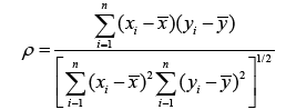
The most common measurement of spatial autocorrelation is the Moran’s autocorrelation coefficient (often denoted as I). It is an extension of Pearson-moment correlation coefficient to a univariate series [31,32]. Recall that Pearson’s correlation (denoted as ρ) between two variables x and y both of length n is:
 (1)
(1)
where and are the sample means of both variables. ρ measures whether, on average, xi and yi are associated. In the study of spatial patterns and processes, it is logically expected that close observations are more likely to be similar than those far apart. It is common to associate a weight with each pair ( xi, xj ) that quantifies this expectation [33]. In its simplest form, these weights will be 1 for close neighbors, and 0 otherwise. The weights are sometimes referred to as a neighboring function with wii set to be 0. Moran’s I can be interpreted as the correlation between variable, x, and the “spatial lag” of x formed by averaging all the values of x for the neighboring areal units (i.e., polygons).
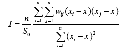
Moran’s autocorrelation coefficient I’s measured by:
 (2)
(2)
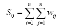
where wij is the weight between observation i and j , and S0 is the
sum of all wij :
 (3)
(3)
Moran’s I varies on a scale between [-1,1]. When the value is close to -1, it means high negative spatial autocorrelation; when the value is close to 0, it means no or minimal autocorrelation; when the value is close to 1, it suggest high positive spatial autocorrelation.
The null hypothesis is that the Spatial Autocorrelation (Moran’s I) is that the data is completely spatial random. If the p-value is not statistically significant, the null hypothesis cannot be rejected. If the p-value is statistically significant, and the z-score is positive, the null hypothesis is rejected. Table 1 shows Moran’s I and its statistical testing results. Almost all the zonal attributes are determined to be spatially dependent.
| Variables | Description | Moran's I | P-Value | Z-Sore | Null hypothesis | Spatially Dependent? |
|---|---|---|---|---|---|---|
| AT | Area Type (CBD, Urban, Suburban, Rural) | 0.8705 | 0.0000 | 37.2544 | Reject | Yes |
| AVGAUTO | Average Auto Owned Per Household | 0.7469 | 0.0000 | 29.0066 | Reject | Yes |
| ACRES | TAZ Area in Acres | 0.5974 | 0.0000 | 23.6038 | Reject | Yes |
| AVGWK | Average Worker Per Household | 0.5387 | 0.0000 | 22.9845 | Reject | Yes |
| EMP_DENSIT | Employment Density | 0.5041 | 0.0000 | 21.4985 | Reject | Yes |
| POP_DENSIT | Population Density | 0.4413 | 0.0000 | 18.5071 | Reject | Yes |
| TOTAL_AUTO | Automobiles in Zone i | 0.2795 | 0.0000 | 12.4357 | Reject | Yes |
| POP | Population in Zone i | 0.2693 | 0.0018 | 11.1823 | Reject | Yes |
| TOTAL_HH | Total Households in Zone i | 0.2688 | 0.0002 | 11.4844 | Reject | Yes |
| TOTAL_EMPL | Total Employment in Zone i | 0.2159 | 0.0000 | 10.0942 | Reject | Yes |
| EMP_M | The medium trip rate employment (Finance, Insurance, Real Estate, Public, Service, Wholesale Trade) in zone i | 0.1874 | 0.0613 | 8.5768 | Accept | No |
| Avg_TRIPSP | Trip Speed Average from Survey Data | 0.1803 | 0.0050 | 7.4908 | Accept | No |
| Avg_CarbEM | Trip Carbon Emission Average from Survey Data | 0.1040 | 0.1040 | 5.2841 | Accept | No |
(Cutoff p-value 0.001)
Table 1: Moran's I and its spatial dependency check.
Candidate spatial cross-sectional models
The general form of spatial cross-sectional model is below:

where:
• WY denotes the endogenous interaction effects among the dependent variables,
• WX the exogenous interaction effects among the independent variables, and
• Wu the interaction effects among the disturbance terms of the different spatial units.
• ρ is called the spatial autoregressive coefficient,
• λ the spatial autocorrelation coefficient, while
• θ represents a K × 1 vector of fixed but unknown parameters.
Figure 3 shows the variations of spatial cross-sectional models with respect to assumptions in the error distribution in the above parameters. Since no predeterminations on the error term distribution can be made, this study tested all the below spatial cross-section models and the best model fits the data will be selected.

Figure 3: The relationships between spatial dependence models for cross-section data.
Results
OLS regression analysis results
Table 2 shows the variables with their coefficient estimates. The R2 (coefficient of determination) gives information about the goodness of fit of a model. In regression, the R2 is a statistical measure of how well the regression line approximates the real data points. An R2 of 1 indicates that the regression line perfectly fits the data. The linear model has a R2 of 0.8002, which suggests that the model is a good fit.
| Variables | Estimate | Std. Error | t | p-value | Pr(>|t|) |
|---|---|---|---|---|---|
| (Intercept) | -1.61E-01 | 1.08E-01 | -1.482 | 0.138675 | |
| ACRES | 7.61E-05 | 4.48E-05 | 1.697 | 0.09016 | . |
| AT | 1.87E-01 | 4.71E-02 | 3.965 | 8.10E-05 | *** |
| POP | 4.57E-04 | 1.01E-04 | 4.535 | 6.80E-06 | *** |
| TOTAL_HH | 4.20E-04 | 2.17E-04 | 1.932 | 0.053826 | . |
| TOTAL_EMPL | -3.78E-05 | 2.48E-05 | -1.52 | 0.128934 | |
| POP_DENSIT | -2.13E-02 | 4.87E-03 | -4.369 | 1.44E-05 | *** |
| EMP_DENSIT | 4.21E-04 | 2.84E-04 | 1.485 | 0.13811 | |
| TOTAL_AUTO | 4.96E-04 | 1.04E-04 | 4.772 | 2.24E-06 | *** |
| EMP_M | 2.40E-01 | 7.07E-02 | 3.39 | 0.00074 | *** |
| AVGWK | 1.58E-01 | 8.50E-02 | 1.862 | 0.062971 | . |
| AVGAUTO | -1.94E-01 | 7.48E-02 | -2.594 | 0.009688 | ** |
| Avg_CarbEM | -7.54E+01 | 2.11E+01 | -3.582 | 0.000365 | *** |
| Avg_TRIPSP | 1.99E-02 | 3.56E-03 | 5.589 | 3.32E-08 | *** |
(Residual standard error: 0.5001 on 679 degrees of freedom Multiple R-squared: 0.8002, Adjusted R-squared: 0.7964 F-statistic: 209.2 on 13 and 679 DF, p-value: <2.2e-16)
Table 2: OLS regression model and coefficients.
Figure 4 is a diagnose plot of the fitted linear model. The first two plots (Residual and Normal Q-Q plots) describe the distribution of the residuals. Ideally, those two plots should be roughly normal. The Outliers (TAZ No. 28, 198, 231 and 669) are shown on the two plots. The scale-location plot is similar to the residuals versus fitted values, but it uses the square root of the standardized residuals. A good fit linear model should show randomness in this plot. The last plot, residuals versus leverage, uses Cook’s distance to identify points which have more influence than other points. Generally these are points that are distant from other points in the data, either for the dependent variable or one or more independent variables. Each observation is represented as a line whose height is indicative of the value of Cook’s distance for that observation. There are no hard and fast rules for interpreting Cook’s distance, but large values (which will be labeled with their observation numbers) represent points, which may require further investigation.

Figure 4: Diagnose plot for OLS regression model.
K-fold cross-validation of the OLS model
K-fold cross validation is one way to improve over the holdout method. The data set is divided into k subsets, and the holdout method is repeated k times. Each time, one of the k subsets is used as the test set and the other k-1 subsets are put together to form a training set. Then the average error across all k trials is computed. The advantage of this method is that it matters less how the data gets divided. Every data point gets to be in a test set exactly once, and gets to be in a training set k-1 times. The variance of the resulting estimate is reduced as k is increased. The disadvantage of this method is that the training algorithm has to be rerun from scratch k times, which means it takes k times as much computation to make an evaluation. A variant of this method is to randomly divide the data into a test and training set k different times. The advantage of doing this is that you can independently choose how large each test set is and how many trials you average over. A common k number for model cross validation is 10. However, since there are 693 TAZs in our dataset, k=9 is used to ensure each “fold” is equal.
Since the data are randomly assigned to a number of ‘folds’. Each fold is removed, in turn, while the remaining data is used to refit the regression model and the deleted observations are predicted. Table 3 shows the residual sum of squares and mean square. Figure 5 is the validation plot showing the removed (folded) vs. fitted data. The validation plot shows a good validation since each removed vs. fitted data flows similar 45 degree line. Overall, the OLS model is validated and it is a good fit.
| Fold | Residual Sum of Squares | Residual Mean Square |
|---|---|---|
| 1 | 21.20 | 0.28 |
| 2 | 17.30 | 0.22 |
| 3 | 21.50 | 0.28 |
| 4 | 11.50 | 0.15 |
| 5 | 11.00 | 0.14 |
| 6 | 24.80 | 0.32 |
| 7 | 26.60 | 0.34 |
| 8 | 22.70 | 0.30 |
| 9 | 23.20 | 0.30 |
| Average | 19.98 | 0.26 |
Table 3: The 9-fold cross validation residuals.

Figure 5: The 9-fold cross-validation results.
Spatial regression analysis results
The spatial regression models are estimated using the maximum likelihood method. Table 4 shows the variable coefficients using the OLS, SAR, SEM, SDM, SDEM, KPM, and MAM. The coefficients that are not spatially dependent (i.e., Avg_CarbEM, Avg_TRIPSP) are quite similar. And the spatially dependent variables have more variations in the coefficient. This is expected because each of the models has different assumptions and is of different forms as shown in Figure 3.
| Coefficients | OLS | SAR | SEM | SDM | SDEM | KPM | MAM |
|---|---|---|---|---|---|---|---|
| (Intercept) | -1.61E-01 | -1.38E-01 | -1.61E-01 | -6.37E-02 | -1.61E-01 | -1.42E-01 | -3.17E-02 |
| ACRES | 7.61E-05 | 5.66E-05 | 7.68E-05 | 2.17E-04 | 7.68E-05 | 7.37E-05 | 2.41E-04 |
| AT | 1.87E-01 | 1.93E-01 | 1.87E-01 | 3.00E-01 | 1.87E-01 | 1.88E-01 | 3.11E-01 |
| POP | 4.57E-04 | 4.59E-04 | 4.57E-04 | 5.50E-04 | 4.57E-04 | 4.75E-04 | 5.77E-04 |
| TOTAL_HH | 4.20E-04 | 4.68E-04 | 4.20E-04 | 6.05E-04 | 4.20E-04 | 4.65E-04 | 6.33E-04 |
| TOTAL_EMPL | -3.78E-05 | -4.22E-05 | -3.78E-05 | -5.08E-05 | -3.78E-05 | -4.19E-05 | -4.96E-05 |
| POP_DENSIT | -2.13E-02 | -2.18E-02 | -2.13E-02 | -2.55E-02 | -2.13E-02 | -2.21E-02 | -2.68E-02 |
| EMP_DENSIT | 4.21E-04 | 3.78E-04 | 4.21E-04 | 3.75E-04 | 4.21E-04 | 3.72E-04 | 3.22E-04 |
| TOTAL_AUTO | 4.96E-04 | 4.78E-04 | 4.95E-04 | 2.56E-04 | 4.95E-04 | 4.56E-04 | 2.08E-04 |
| EMP_M | 2.40E-01 | 2.36E-01 | 2.40E-01 | 1.87E-01 | 2.40E-01 | 2.35E-01 | 1.83E-01 |
| AVGWK | 1.58E-01 | 1.70E-01 | 1.59E-01 | 1.91E-01 | 1.59E-01 | 1.74E-01 | 1.84E-01 |
| AVGAUTO | -1.94E-01 | -1.62E-01 | -1.94E-01 | -8.03E-02 | -1.94E-01 | -1.65E-01 | -6.22E-02 |
| Avg_CarbEM | -7.54E+01 | -7.54E+01 | -7.54E+01 | -7.58E+01 | -7.54E+01 | -7.47E+01 | -7.46E+01 |
| Avg_TRIPSP | 1.99E-02 | 2.02E-02 | 1.99E-02 | 1.98E-02 | 1.99E-02 | 1.99E-02 | 1.96E-0 |
(OLS: Ordinary Least Square; SAR: Spatial Autoregressive Model; SEM: Spatial Error Model; SDM: Spatial Durbin Model; SDEM: Spatial Durbin Error Model; KPM: Kelejian Prucha Model; MAM: Manski Model)
Table 4: Model coefficients comparison for OLS, SAR, SEM and SDM models.
Goodness of fit measures for candidate models
The goodness of fit measures in spatial regression models is slightly more complex due to the lack of standard measures such as R2. However, commonly used goodness of fit measures is the information-based measures. The information-based goodness of fit measures utilizes several model performance measures and rank based on the values. The model with the lowest rank is considered a better fit than others. Table 5 shows the information based measures and their ranks for OLS, SAR, SEM, SDM, SDEM, KPM and MAM models. This ranking utilized AIC, Log Likelihood and Moran’s I on Residuals as measures. For all three criteria, smaller values are better. Therefore, the SDEM model has the lowest summation of ranks and it fits the data better.
| Model Type | AIC | Rank | Log Likelihood | Rank | Moran’s I on Residuals | Rank | Total Rank |
|---|---|---|---|---|---|---|---|
| Ordinary Least Square (OLS) | 1092.5 | 4 | -533.2 | 5 | +0.026397503 | 5 | 14 |
| Spatial Autoregressive Model (SAR) | 1088.4 | 3 | -530.2 | 3 | +0.056595454 | 6 | 12 |
| Spatial Error Model (SEM) | 1093.1 | 5 | -532.6 | 4 | -0.000634720 | 1 | 10 |
| Spatial Durbin Model (SDM) | 1065.3 | 2 | -507.7 | 2 | -0.008763889 | 4 | 8 |
| Spatial Durbin Error Model (SDEM) | 1064.1 | 1 | -532.6 | 4 | -0.000634720 | 1 | 6 |
| Kelejian-Prucha Model (KPM) | N/A | 3.5 | N/A | 3.5 | -0.000340069 | 2 | 9 |
| Manski Model (MAM) | 1093.8 | 5 | -506.4 | 1 | -0.0052871289 | 3 | 9 |
Table 5: Information-based measure of fit for spatial models.
Discussion
A spatial regression-based modeling framework was developed based on finding the minimal model residuals and multiple informationbased measures of fit. The goodness of fit measures in spatial regression models is slightly more complex due to the lack of standard measures such as the R2. However, a common goodness of fit measures is the information-based measures. The information-based goodness of fit measures utilizes several model performance measures and ranks based on the values. The model with the lowest rank is considered a better fit than others. The information-based measures and their ranks for OLS, SAR, SEM, SDM, SDEM, KPM and MAM models are summarized and presented.
OLS model has an R2 (coefficient of determination) of 0.8, which is a good fit. However, when examining the residuals on diagnosis plots, it was found that the residuals are still spatially correlated. This suggests that spatial models can fit the data better and reduce the residual spatial correlation. After performing spatial regressions, the informationbased measure of fit based on AIC, log likelihood and Moran’s I on residuals are compared and the best model fitting the given dataset is the Spatial Durbin Error Model. The SDEM has the lowest AIC and Moran’s I on residuals compared to other candidate models.
This study has provided a proof of concept for the proposed methodology and solid foundation for the modeling land use changes, and GHG emission analysis. It has been proven that the proposed method has the capability to reveal the dynamic linkage between land use, transportation, and emissions. The findings from this research provide insights on how land-uses planning alternatives built on adopted policies and enforced development regulations correlate with travel patterns and their sequential GHG emissions. The level of specificity, such as the land use change and GHG emission analysis presented in this study enables more data and indicators to be developed. Such data and indicators can be incorporated into decision makers’ plans, policies and ultimately regulations and its possible integration with project level review processes.
Conclusion
While the results from this study offer specific recommendations as to which types of land use planning policy practices are most highly associated with a higher amount of VMT, GHG emissions, there are also some potential to reveal policy impacts that can be applied to integrated land use and transportation sustainability practices. The results of this research are expected to add to the existing body of knowledge to enable faster and easier methods of examining the impact of adaptive planning strategies on alleviating the effects of household travel GHG emissions. The spatial cross-sectional regression model is developed through the integration of actual and scenario based land use visioning and planning, demographical changes, transportation emission analysis, and computer forecasting and evaluation of future scenarios. This research makes it possible to assess the household travel GHG footprint and provides models, data for possible GHG emission mitigation through land use policies and changes. Although the results may be pertaining to the specific dataset but it helps transportation decision makers to better connect the land use development and its related household socioeconomics with their GHG emission characteristics. Particular, the household travel GHG emission quantification results made its contribution to the current body of knowledge on the following: (1) provides accurate GHG emission results by using the best available traffic activity data inputs (VSP distributions) for emission modeling; (2) provides connections between household socioeconomics and their travel GHG footprint. The research suggests important potential to provide solid grounds for analyzing, modeling of sustainable community strategies, adaptive planning policies, and many other policy-making applications.
Acknowledgement
The authors are appreciative of the support by U.S. EPA and Ohio-Kentucky- Indiana Regional Council of Governments. Any opinions expressed in this paper are the author(s)’s point of view and do not necessarily reflect the views of the Agency.
References
- USEPA. Fast Facts: U.S. Transportation sector greenhouse gas emissions 1900-2010. Facts EPA 420-F12-063, United States Environmental Protection Agency, Washington, DC.
- USEPA (2012) Using MOVES to prepare emission inventories in state implementation plans and transportation conformity. Washington DC.
- USEPA (2010) Transportation conformity guidance for quantitative hot-spot analyses in PM2.5 and PM10 nonattainment and maintenance areas. Technical guidance EPA-420-B-10-040, USEPA, Washington, DC.
- FHWA (2010) Transportation conformity: A basic guide for state and local officials. Washington DC.
- Guohua S, Lei Y, Ziqianli W (2008) A practical modeling approach for evaluation of fuel efficiency for road traffic. Transportation Research Board Annual Meeting.
- Frey H, Nagui R, Haibo Z (2008) Link-based emission factors for heavy-duty diesel trucks based on real-world data. TRR: Journal of the Transportation Research Board 2058: 23-32.
- Fulper`C, Hart C, Warila J, Koupal J, Kishan S, et al. (2011) Development of real-world data for MOVES development: The Houston Drayage activity characterization study. Transportation Research Annual Meeting.
- Yao Z, Wei H, Perugu H, Liu H, Li Z (2014) Sensitivity analysis of project level MOVES running emission rates for light and heavy duty vehicles. JTTE 1: 81-96.
- Harikishan P, Heng W, Zhuo Y (2016) Integrated data-driven modeling to estimate PM 2.5 pollution from heavy-duty truck transportation activity over metropolitan area. Transportation Research Part D: Transport and Environment 46: 114-127.
- Zhuo Y, Heng W, Hao L, Zhixia L (2013) Statistical vehicle specific power profiling for urban freeways. Elsevier.
- Robinsson R, Edgar V, Paula R, Eduardo B (2016). Influence of driving patterns on vehicle emissions: A case study for Latin American cities. Transportation Research Part D: Transport and Environment 43: 192-206.
- William B, Wayne S, Shauna H, Randall G (2000) Modeling regional mobile source emissions in a geographic information system framework. Transportation Research Part C: Emerging Technologies 8: 205-229.
- Bhat C, Conoor S, Nerella S (2003) GIS-integrated traffic input models for mobile-source emissions analysis. Texas Department of Transportation, Austin.
- Mittal N, Golias M, Boile M, Spasovic L, Ozbay K (2004) Estimating truck volumes on state highways – A statistical approach. Transportation Research Board Annual Meeting.
- Wang H, Jang K, Chan CY (2010) Analysis and Multi-level modeling of truck freight Demand. Strategic Highway Research Program 2 (SHRP2) Freight Modeling and Data Symposium.
- Elhorst JP (2010) Spatial panel model. Handbook of Applied Spatial Analysis. Springer Berlin Heidelberg, Berlin.
- Frazier C, Kockelman KM (2006) Spatial Econometric models for panel data: Incorporating spatial and temporal data. TRR: Journal of the Transportation Research Board 1902: 80-90.
- Wang Y, Kockelman K, Wang X (2012) Anticipation of land use change through use of geographically weighted regression models for discrete response. TRR: Journal of the Transportation Research Board 111-123.
- Wang Y, Kockelman K, Damien P (2013) A spatial autoregressive multinomial probit model for anticipating land-use change in Austin, Texas. Ann Reg Sci.
- Zhou B, Kockelman K (2008) Neighborhood impacts on land use change: a multinomial logit model of spatial relationships. Ann Reg Sci 42: 321-340.
- Zhou B, Kockelman K (2009) Predicting the distribution of households and employment: a seemingly unrelated regression model with two spatial processes. J Trans Geogr 17: 369–376.
- Parent O, LeSage J (2010) A spatial dynamic panel model with random effects applied to commuting times. Transportation Research Part B: Methodological 44: 633-645.
- Perugu H, Wei H, Rohne A (2012) Modeling roadway link PM2.5 emissions with accurate truck activity estimate for regional transportation conformity analysis. TRR: Journal of the Transportation Research Board 2270: 87-95.
- Perugu H, Wei H, Yao Z (2013) An improved methodology for modeling truck contribution to regional air quality. In 14th TRB National Transportation Planning Applications Conference, Columbus.
- Perugu H, Wei H, Yao Z (2014) Modeling truck activity using short-term traffic counts for reliable estimation of heavy-duty truck emissions in urban areas. Transportation Research Board Annual Meeting, Washington DC.
- Yao Z, Wei H, Wang X, Liu H, Yang JY (2014). Scenario-based carbon footprint inventory tool for urban sustainable development decision support: The Cincinnati case study. Transportation Research Board 93rd Annual Meeting, Washington DC.
- Kockelman KM, Frazier C (2005) Spatial econometric models for panel data�?�: Incorporating spatial and temporal data. TRR: Journal of the Transportation Research Board 80-90.
- Chakir R, Gallo JL (2013) Predicting land use allocation in France: A spatial panel data analysis. Ecological Economics 92: 114-125.
- Perugu H, Wei H, Rohne A (2012) Modeling roadway link pm2.5 emissions with accurate truck activity estimate for regional transportation conformity analysis. TRR: Journal of the Transportation Research Board 2270: 87-95.
- Tobler WR (2016) A computer movie simulating urban growth in the Detroit region. Economic Geography 46: 234-240.
- David CA, Ord (1973) JK Spatial autocorrelation. London.
- Moran PAP (1950) Notes on continuous stochastic phenomena. Biometrika 37: 17-23.
- David CA, Ord JK (1981) Spatial and temporal analysis: autocorrelation in space and time. Quantitative Geography: A British View. Routledge & Kegan Paul, London.
Relevant Topics
Recommended Journals
Article Tools
Article Usage
- Total views: 3981
- [From(publication date):
April-2017 - Apr 03, 2025] - Breakdown by view type
- HTML page views : 3148
- PDF downloads : 833