A Data-Driven Approach for Accurate Estimation and Visualization of Energy Savings from Advanced Lighting Controls
Received: 11-Nov-2017 / Accepted Date: 15-Nov-2017 / Published Date: 22-Nov-2017 DOI: 10.4172/2576-1463.1000177
Abstract
Despite occupancy-based switching and daylight-based dimming controls being widely believed to have tremendous energy saving potential, there is often a lot of variability in the actual savings across customer sites. A major challenge in a reliable, site-specific assessment of these advanced lighting controls is the skew associated with time-logging using a low-power clock. We develop a robust analytical approach based on grid-search optimization and linear regression to correct the clock skew by exploiting the information stored in the cyclical nature of occupancy patterns in commercial buildings. We provide independent validation of the results using illuminance data to illustrate the strength of our approach. We also conduct comprehensive sensitivity analyses of the results by varying the assumptions about the underlying parameters values. Our results demonstrate that believable visualizations and reliable savings estimates can be generated using a low-power clock and a set of data-driven algorithms and analytics.
Keywords: Data loggers; Occupancy-based switching; Daylight harvesting; Clock skew correction; RC oscillator clock; Grid-search optimization; Linear regression
Introduction
Occupancy sensors are sensing devices commonly connected to a room’s lighting (and sometimes also to heating, ventilation and airconditioning (HVAC) systems), which shut down these services when the space is unoccupied. Occupancy sensors for lighting control use infrared (IR) or acoustic technology, or a combination of the two. The location and field of view of the sensor are important determinants of its effectiveness. Most systems incorporate a delay time before switching. If the sensor detects no motion for the entire delay time then the lights are switched off. Occupancy sensing technologies have been widely studied in literature [1-5]. Savings potential of the order of 30% to 50% has often been estimated by switching off the light when a space is unoccupied [3].
Daylight harvesting is a type of lighting control that is typically designed to maintain a minimum recommended light level by reducing the use of artificial light when natural daylight is available. The daylight harvesting techniques rely on light level data collected from a photosensor such as a photo-diode. Daylight harvesting technologies have also been extensively studied literature [6-10]. Savings potential of the order of 20% to 60% has been estimated for daylight harvesting-based dimming controls [7].
Materials And Methods
Several commercial products are available in the market, which aim to reduce the lighting energy consumption of indoor spaces by combining the occupancy sensing and daylight harvesting techniques. Examples include Leviton’s Universal Vacancy/Occupancy Sensors, Acuity’s Sensor Switch, WattStopper’s wall switch sensors, etc. The OccuSwitch Wireless Control System by Philips is one such commercial product using a variant of the occupancy sensing and daylight harvesting technology.
Philips occuswitch wireless system
The Philips OccuSwitch Wireless Control System senses occupancy and light level to automatically turn lights off in an unoccupied space and to dim the artificial lights in a space in proportion to the daylight. The system consists of two main components: (1) a wall mounted dimmer switch and (2) a battery-operated ceiling-mounted combination of photo and occupancy sensor, interconnected by ZigBee PRO wireless technology. Some of the important features of this OccuSwitch system are as follows:
• Motion detection: It uses a passive infrared (PIR) sensor technology to detect motion and an advanced logic to identify major and minor motions. The system adapts to accommodate varying user occupancy patterns to automatically adjust the shut-off time delay. Its detection technology with autocalibrated sensitivity helps avoid false “on” triggers. The sensors include an adjustable rotating shield which enables field of view adjustments for occupancy detection.
• Light level detection: The light level reporting frequency is dynamically adapted to save battery energy. The reporting interval is longer when the space is unoccupied or when the light level is stable. But the sensor reports immediately when the light level changes by more than a predetermined threshold. Thus, the system quickly responds to changes in the environment while preserving battery energy.
• Coverage: Its design can support up to ten sensors and switches (in any combination) in a single system to maximize and expand the system coverage.
• Communication system: The occupancy sensor detects motion and the photo-sensor measures the light level. These are then communicated to the dimmer switch over the radio interface. Its wireless communication system automatically selects the best available channel to provide secure, reliable communication between devices and automatically switches between two different antennas to improve/restore communication. Its transceiver is designed to maximize gain and minimize losses between transmitter and receiver to enhance the range and reduce the signal attenuation. The user can also change the communication channel through installer settings to mitigate interference. All messages are encrypted using a 128-bit advanced encryption standard (AES) algorithm with unique keys.
• Power source: Battery lifetime is estimated to be more than 7 years.
• User interface: It has Traffic LED Indicator (red-yellow-green) to provide instant feedback to the users on the system status and uses a USB interface to enable quick software upgrades in the field.
Occuswitch data logger
While the advanced lighting controls based on occupancy sensing and daylight harvesting, such as the OccuSwitch system from Philips, have the potential to reduce lighting energy consumption by 30% to 50% in commercial buildings, the results are found to be highly variable across sites [1,3]. Therefore, there is a need to accurately quantify the actual savings potential for specific buildings, offices and rooms. These calculations need to be performed taking into account the actual usage patterns, occupancy behavior, geometry, geography, climate and type of use of individual indoor spaces. Performing these computations for the specific indoor spaces can help a lighting control system manufacturer convince the users of the benefits of installing advanced lighting controls such as occupancy sensing and daylight harvesting. A strong business case for adopting these systems can only be made on the basis of the savings potential for that specific customer site. A tool that can effectively quantify the spatio-temporal patterns in occupancy, usage and energy consumption can also be a great aid for other purposes such as energy auditing. In addition to accurate logging and estimation, some of the other desirable features in any such product would include portability, easy mounting, quick setup, absence of wiring and low cost. These portable devices do not have to be in physical contact of high voltage wires. As a result, they can be installed by anyone as opposed to the clamp-on power meters which can only be installed by licensed electricians and hence incur higher costs. Various commercial products have been developed to address this challenge by different companies selling lighting controls. The indoor standalone OccuSwitch Data Logger by Philips is an example of such devices.
Philips OccuSwitch Data Logger is a standalone wall/ceiling mountable unit that monitors the light level (illuminance) and occupancy status of the room continually. It consists of a passive infrared sensor which works as motion detector, a photo-sensor that measures the amount of light in the room. It also contains a clock for logging the relative timestamps and a battery to power the system. At periodic intervals, the logger records a timestamp (recorded by the clocks), illuminance (recorded by the photo-sensor) and occupancy status (recorded by the PIR motion detector). After the installation period (of about one to three months) the logger is removed from wall and connected to a PC through a USB port. An accompanying software program downloads the data, performs numerical analysis and then estimates the energy savings potential.
Neves-Silva et al. [11] provide the details of the framework for a software tool that models the energy consumption from monitored data on building infrastructure usage, predicts consumption under alternative scenarios and supports the decision-making process providing investment recommendations and installation plans. The authors of this study acknowledge that, as noted by Parker et al. [12] and Vieira [13], the behavior of occupants of a building can have a very large impact on energy consumption. Therefore, they make a strong case for sensing and energy metering at the actual facility where installation of an energy-efficient technology is being considered. The same argument applies for our efforts towards estimating the savings through the occupancy-based switching and daylight harvesting-based dimming of lights. However, these prior research studies do not address the challenges involved in effective use of raw data collected through inexpensive sensors such as OccuSwitch Data Loggers. They instead assume the availability of clean sensor and metering data, focusing on the recommendation of the most appropriate configuration of technologies and devices tailored to the specific needs of individual buildings, rooms and users.
Problem Statement
The OccuSwitch Data Logger (or Data Logger for short) consists of a low-accuracy, low-power clock made up of an RC (Resistor- Capacitor) Oscillator circuit. This clock is known to have a skew of the order of up to 15 minutes (plus or minus) per day. The skew is usually constant for each clock at a given temperature, but differs across different clocks and different temperatures. Given the indoor usage of the data loggers, we can ignore the variance in skew due to temperature fluctuations without introducing too much error. The main advantage of using this low-accuracy clock is that it uses less power and hence guarantees a longer battery life.
In addition to the RC clock, the loggers also contain a much more accurate Quartz crystal clock with accuracies of the order of 10 parts per million (ppm) or so. It is, however, a lot more power-intensive. So the logger uses the accurate clocks sporadically. The accurate clock is used only during a part of the occupied time periods where accurate time measurements are especially important. For most of the other time, the low-power RC clock is used to measure relative timestamps. Each time the logger switches from more accurate to less accurate clock and vice versa, there is also likely to be a very small handoff delay. The timestamps for all data entries are compared with the timestamp of the time when the logger is connected to a PC at the end of the data collection period and the actual time corresponding to each data entry are then calculated based on the relative timestamp value. When the room is unoccupied, the RC clock is used almost exclusively, while the Quartz clock is used for a part of the time when the room is occupied. Due to these differences, the error in recorded times accumulates at different rates during the occupied and the unoccupied time periods.
Due to the errors in time measurement, the timestamps recorded with the data entries are different from the actual times when those data were recorded. Over a three month period, the difference between actual and recoded timestamps can be as high as two to three days. Therefore, a posterior correction is indispensable in order to perform any informed decisions based on this data and to visualize this data effectively. The available data consists of occupancy and illuminance. Illuminance is affected by artificial light as well as daylight. The latter contains information about the time-of-day, but is difficult to separate from the artificial light and is further affected by issues such as room orientation, window location, use of blinds, cloud cover etc. Occupancy, on the other hand, is usually well tied to the occupants’ work schedules. Most rooms in commercial and office buildings are a lot more heavily used during the weekdays than during the nights and weekends. Furthermore, these usage patterns are often highly cyclical and repetitive in nature. Therefore, they constitute a useful input for any correction technique. We use the occupancy information to estimate the clock skew and use the illuminance information as an independent source of validation data for the clock skew estimation. Exploiting the occupancy patterns in commercial or office buildings for correcting the clock skew constitutes an interesting research challenge. This problem can be formally represented as follows:


where,
T: Number of data entries corresponding to an occupancy-related event, that is, occupancy changing from unoccupied to occupied (from 0 to 1) or vice versa.
N: Number of data loggers
τtn : Measured time corresponding to the tth data entry for nth logger
otn : Occupancy value immediately after an occupancy-related event corresponding to the tth data entry for nth logger, otn ∈ {0, 1}

Where,
 : Estimate of clock skew for the nth logger, when occupied (note that the Quartz clock is being used for a part of the occupied time),
 : Estimate of clock skew for the nth logger, when unoccupied (note that the RC clock is used for the entire duration of the unoccupied time).
Model
This model exploits the patterns in the office space usage of the occupants of an office. In reality, during the time for which the room is occupied, both the accurate and the less accurate clock is used for part of the time, the decision to use a particular clock during a certain part of the occupied time is dependent of a complex internal logic, which is difficult to model accurately. Instead, we assume that the clock skew during the occupied time has a constant average value. The accuracy of our results justifies this assumption. During the unoccupied state, the less accurate clock is used to preserve battery life. Therefore we can safely assume a constant skew during the unoccupied periods. All time in the model below is measured backward, with time 0 representing the point in time when the study period ended and the logger was removed from the ceiling and connected to a PC through a USB port. The timestamp for each data entry is the difference between the time when that particular data was recorded and the time 0 representing the time when the logger is connected to a PC.


Clock skew is defined as a multiplicative factor that modifies the time measured by the logger. A factor>1 (<1) means that the measured time moves faster (slower) than actual time by that factor.
In addition, there might be some day-specific factors that might affect the schedules of all the occupants of a building similarly. For example, all (or most) occupants might want to leave earlier than usual on a Friday, or arrive later than usual on a Monday, or leave especially early on the Wednesday before Thanksgiving Day in the U.S., etc. We call this a day-specific additive bias, which is assumed to be constant across all occupants.


Furthermore, there could be some individual-specific factors. For example, some individuals have a tendency to work until late and therefore they stay longer in the office than others. These factors are specific to an individual occupant and hence they can be assumed to remain constant across time for a specific logger (that is, for the occupant(s) of a room containing a specific logger). We call this a personal additive bias, which is assumed to be constant across all loggers.


Under this general model, the workday start and end time for room containing nth logger on dth day is as follows.
 (1)
(1)
 (2)
(2)
Where,
 and
and  are the standard (or typical) values of workday start and end times on each day, e.g. 8 am and 5 pm respectively. ε'dn and γ'dn are random variables (with zero means) representing errors in this model. These can be considered as the cumulative effects of all the other factors affecting the work-day start and end times.
For the room with the nth logger, let fdn be the occupied fraction of the measured time from the start time of dth work-day until the end of the study period. Also, for the room with the nth logger, let gdn be the occupied fraction of the measured time from the end time of dth workday until the end of the study period.
Thus,  is the length of the measured occupied time and
  is the length of the measured unoccupied time from the start of dth work-day for the occupant of the room with the nth logger. So,
  is the length of the actual occupied time and
  is the length of the actual unoccupied time from the start of dth work-day for the occupant of the room with the nth logger. As a result, the total actual duration of time from the start of dth work-day till the end of the study for the occupant of the room with the nth logger is:

where,  are the inverses of the clock skews,
  and
and  respectively, for all n ∈{1..N}
Therefore,
 (3)
(3)
and by an analogous argument we can show that,
 (4)
(4)
From equations 1, 2, 3 and 4 we get,
 (5)
(5)
And
 (6)
(6)
Upon rearranging terms we get,

and

Where,

So, the overall model is as follows: 
 (7)
(7)
and
 (8)
(8)
The values of  ,
,  , fdn and gdn are known because they can be directly measured. The values of
  and
and  can also be ascertained based on our knowledge of the typical working hours. Alternatively, we could also consider asking the user to provide the typical working hours of the office as one of the user-provided inputs, to obtain more accurate estimation results.
So the parameters to be estimated are,  , and
, and  , in the most general case. So, for this general model, the total number of unknown parameters=4N+2D and total number of observations=2ND. In reality, the number of unknown parameters is likely to be lower than this if we make some further simplifying assumptions as described in the next section.
Data Description
The data is collected from an office building at one of the customer sites in the United Kingdom. There were 22 loggers used for this study. All the loggers were installed in private office spaces on a single floor, one logger per private office. Out of these 22 loggers, data from one was tagged as “Battery Failure” and therefore was excluded from all the computations. So we had usable data from 21 loggers over the study period.
The data used for the estimation process was contained in comma separated variable files (.csv files) each containing the data downloaded from one logger. The data was over a time period of approximately three and half months (103 days: starting from December 5th 2011 to March 16th 2012). However, the actual number of days with data was much fewer. Most of the useful observations are concentrated in the 42 days period between December 7th 2011 and January 17th 2012. This is likely so because at this customer site, the customer decided to remove the loggers from their respective locations but did not connect them to a PC for around 2 months. This created additional challenges in getting useful information out of the data.
Each comma separated variable file consisted of five columns:
1. Time: Time when that observation was recorded. Measured in year, month, day-of-month, hour, minute and second.
2. Occupancy: A 0/1 binary variable indicating whether or not the occupancy sensor detected the room as occupied. Data can be recorded for various reasons, including a change in occupancy value. In records where the observation indicates a change in occupancy, the occupancy column contains the occupancy value just after the change had happened. e.g. when the room’s occupancy status changes to occupied from previously unoccupied state, the Occupancy column records a 1.
3. Illuminance Level: Illuminance measured by the photo-sensor in Lux.
4. Light State: A 0/1 binary variable indicating the light state estimated by a pre-existing algorithm using the time series of illuminance data. A light state value of 1 means that the artificial light is on and 0 means off.
5. Reason: The reason why that particular observation was retained. In order to minimize the storage needs on the chip, the loggers store only a relevant subset of all the observations. As a result, the sensor readings are not continuous, but rather are quantized. Only those readings are logged which correspond to a timestamp where something worth noting has happened. An observation can be logged and retained for one of the following six reasons:
α. OCCUPANCY: If the occupancy state changed from 0 to 1 or from 1 to 0.
β. FAST: If the photo-sensor detected a rapid change in illuminance level, which is usually an indication of artificial light being turned on or off.
χ. EXTREME: If a local maximum or a local minimum in illuminance level is observed. Here, a local maximum (minimum, respectively), in a time series data like this, is defined as the maximum (minimum, respectively) value of the measured entity in a small time period containing the time when that value was measured. In other words, all values measured at times just before and just after that value was measured should be less than or equal to (greater than or equal to, respectively) that value.
δ. LARGE: If a large (to be contrasted against a fast) change is observed in the illuminance level.
ε. CONSTANT: If no observation is recorded for a long period of relatively little activity and no significant changes in illuminance level, then a few intermediate observations are recorded to demarcate the periods of constant illuminance from those of slowly changing illuminance.
Φ. DUPLICATE: Some additional observations to improve the computations and visualization.
In addition, each data file also contains (1) one value for “HoldTime” i.e. the time-off delay in milliseconds and (2) one value for “Threshold” i.e. the minimum recommended illuminance level on the photosensor in Lux. The minimum recommended illuminance level is the amount of illuminance that is deemed to be sufficient for the occupants to perform their desired activities satisfactorily and comfortably. An example of the data file is shown in Table 1, which displays a snapshot of the top 20 rows of one such data file.
| Time | Occupancy | Illuminance level | Light state | Reason | Hold time | Threshold |
|---|---|---|---|---|---|---|
| 12/12/2011 3:31 | 1 | 37 | 1 | OCCUPANCY | 978000 | 37 |
| 12/12/2011 3:46 | 1 | 37 | 1 | FAST | ||
| 12/12/2011 3:46 | 1 | 61 | 1 | FAST | ||
| 12/12/2011 3:47 | 1 | 37 | 1 | EXTREME | ||
| 12/12/2011 3:47 | 1 | 49 | 1 | FAST | ||
| 12/12/2011 4:03 | 1 | 37 | 1 | FAST | ||
| 12/12/2011 4:03 | 1 | 12 | 1 | DUPLICATE | ||
| 12/12/2011 4:03 | 1 | 12 | 0 | FAST | ||
| 12/12/2011 4:04 | 1 | 12 | 0 | DUPLICATE | ||
| 12/12/2011 4:04 | 0 | 12 | 0 | OCCUPANCY | ||
| 12/12/2011 6:36 | 0 | 0 | 0 | FAST | ||
| 12/12/2011 6:36 | 0 | 0 | 0 | DUPLICATE | ||
| 12/12/2011 6:36 | 1 | 0 | 0 | OCCUPANCY | ||
| 12/12/2011 6:37 | 1 | 37 | 0 | EXTREME | ||
| 12/12/2011 6:51 | 1 | 37 | 0 | FAST | ||
| 12/12/2011 6:51 | 1 | 12 | 0 | FAST | ||
| 12/12/2011 6:53 | 1 | 12 | 0 | DUPLICATE | ||
| 12/12/2011 6:53 | 0 | 12 | 0 | OCCUPANCY | ||
| 12/12/2011 13:25 | 0 | 0 | 0 | EXTREME |
Table 1: A snapshot of a data file.
Raw data analysis
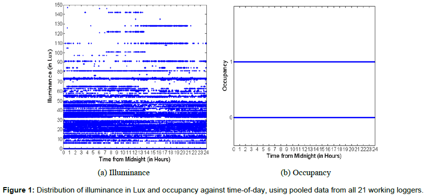
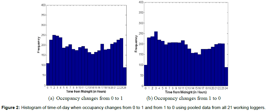
Figures 1a, 1b shows the aggregated occupancy patterns and illuminance levels, respectively, recorded by all 21 working loggers, against time-of-day in hours. Similarly, Figures 2a, 2b show the distribution across time-of-day of all the instances when the occupancy changes from 0 to 1 and from 1 to 0 respectively, for all 21 working loggers. The time-of-day values are the raw measurements as measured by the loggers, uncorrected for clock skew. Figures 1 and 2 demonstrate how the raw data is almost uniformly distributed across different timesof- the-day. This temporal distribution clearly shows that this data is highly unusable in its current form for any analysis and visualization purposes. In fact, the distribution of points on horizontal lines representing occupancy=0 and occupancy=1 in Figure 1b is so uniform that they appear to be parts of a continuous line. This motivates the clock skew correction efforts in the subsequent sections.
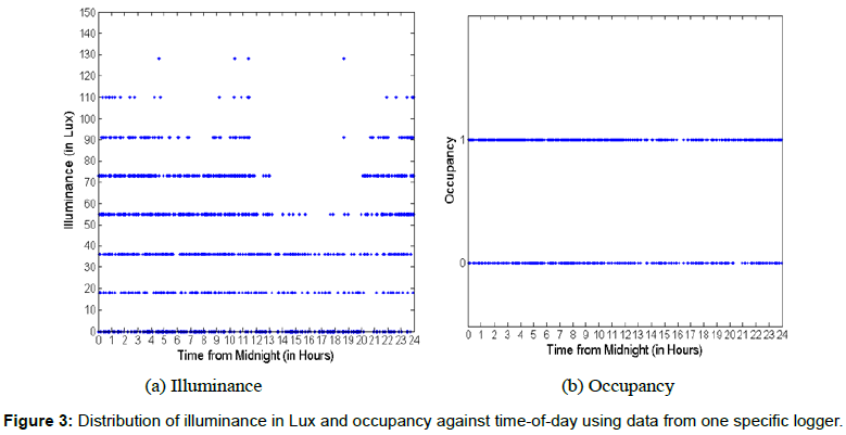
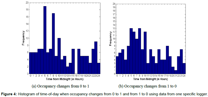
Figures 3a, 3b and 4a, 4b display the same four charts displayed in Figures 1a, 1b and 2a, 2b respectively, but now for one specific logger rather than for the aggregation of data from all 21 loggers. As can be observed from inspection of Figures 3a, 3b and 4a, 4b, the conclusions drawn earlier based on aggregate data do not change. It is still very difficult to make any sense out of this data because the occupancy and illuminance data is distributed seemingly randomly across the day.
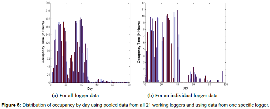
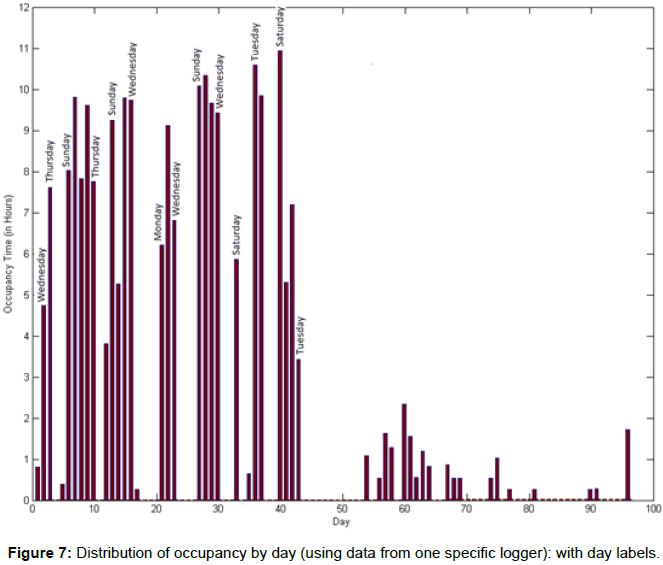
Figures 5a, 5b display the distribution of occupancy by day, for aggregated data from all loggers and for data from a specific logger, respectively. If we had accurate timestamp data, each of these figures should have shown seven-day cycles with five continuous days of high occupancy followed by two days of low or zero occupancy. This is because of the fact that most people tend to work for many more hours during an average weekday than during an average weekend day and hence occupy their office rooms longer on weekdays than on weekends. It is interesting to note that even though Figure 5a contains some cyclical patterns, but it is still very difficult to identify the five-day weeks in most cases. This is due to the aggregation of data with different skew rates. This is clear when we look at Figure 5b. The cycles in Figure 5b are a lot more prominent and are easy to group into five-day periods, which correspond to weekdays in each week. This gives us insight into how we can approach the problem of clock skew correction. It is interesting to note that for both Figures 5a, 5b, there is very little data beyond Day 50 or so. This was found to be the case for all the loggers from which we collected the data. We suspect that the loggers were removed from ceiling around that time and stored for some more days before connecting to a PC and retrieving the data from them. This conjecture seems reasonable especially because we found very little data of any kind beyond a certain day for each of the 21 working loggers.
Solution Algorithm
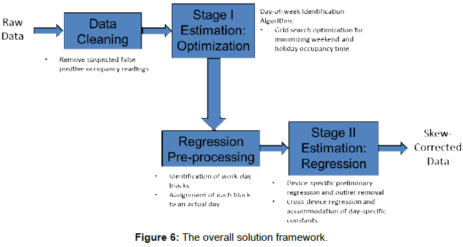
The overall solution framework is presented in Figure 6. As the first step of the algorithm, we performed data cleaning, where we removed false triggers. These correspond to data entries where the occupancy sensor shows an occupancy value of 1 even though the room is, in reality, unoccupied and vice-versa. This can happen due to various reasons including people passing by close to the room entrance, some quick fluctuations in the room’s heating patterns, maintenance personnel entering the room briefly during night time (to remove trash etc.), room occupants remaining steady for a long period of time, or simply due to sensor inaccuracies. Some of these false alarms can be easily detected by identifying occupancy periods which are exactly equal to the time-off delay (hold time) period in duration, indicating instantaneous movement detection but nothing after that instance. So the first step of the solution algorithm is vital because it removes such false triggers. Note that the entire data cleaning step and all other steps in the estimation algorithm are fully automated and has been embedded into our final software product. We used our data miningbased insights to fine-tune to algorithmic parameters.
Even after the data cleaning step, the linear regression model presented in Section 3 by equations (7) and (8) cannot be used directly for estimating the clock skew. This is primarily because based on the raw timestamp data it is very difficult to identify which day each observation belongs to. Hence we cannot directly calculate  and
and  (i.e., the durations of time periods from the typical start time of each day till the end of the study period and the duration of time periods from the typical end time of each day till the end of the study period), which are necessary input data elements to run the regression models given by equations (7) and (8) in Section 3. If we annotate the bar chart in Figure 5b with names of weekdays (as shown in Figure 7) the cyclical patterns do not match with weekdays in the raw data. For example, looking at Figure 7, some weeks seem to be starting on a Wednesday, some on a Sunday, some on a Saturday, etc. So the first step towards identifying the correct times is to identify the correct day (of the week) corresponding to the data entries. Therefore, after data cleaning, our next step in skew correction involves a coarser level correction where the output of the task is the correct value of day for each data entry.
Day-of-week identification algorithm
For this task, we rely on the previously stated assumption that office rooms tend to be less occupied on weekends and public holidays as compared to that on working days. Therefore, we formulate the problem as an optimization problem where the objective function is to minimize the amount of time for which the room was occupied on holidays (that is, weekend days and public holidays). In this first step, we are looking for only an approximate estimate of the skew rate so that we get the day correct. Therefore, in order to simplify the estimation process, we estimate the skew rate for each logger separately rather than pooling in the data from all 21 loggers. Also, we assume a single skew rate value for each logger, rather than estimating one skew rate value for occupied duration and one value for unoccupied duration as we suggested in the general problem formulation described by equations (7) and (8). So the simplified problem for a specific logger n, is described formally below:

We formulate the problem as follows:
First we note that, as mentioned earlier, all time in the model is measured backward, with time 0 representing the point in time when the study period ended and the logger was removed from the ceiling and connected to a PC through a USB port. Let Ln represent the true time in seconds since the last midnight (as per the clock in the PC) when the study period ended for a logger number n. A example, if the study period ended at 3:30 pm time on some day then, L = (12 +3)*3600 +30*60 = 55,800 seconds. Let us denote the last day of the study period as day 0. Let H denote the set of integers representing days that fall on weekends and public holidays during the study period when measured backward from the last day of the study period. As mentioned earlier, the input data is represented as  . Let us denote the approximate clock skew to be estimated as b.
 and
and  are the three main inputs of this optimization problem, while b is the only output of the model. The following expression represents the union of all the time intervals when the room was occupied according to the raw times measured by the logger.

If the logger’s average skew rate is b, then this can be written in terms of the union of all the time intervals when the room was occupied according to the skew-corrected time measurements as follows:
 The union of all time intervals corresponding to the weekends and holidays according to accurate time measurements is as follows:

Note that all times are measured backward from the end of the study period. The number 86400 equals the number of seconds in a day (24*60*60). The set of time intervals (according to skew-corrected accurate time) that fell on weekends or public holidays when the room containing the nth logger is occupied is given by the following expression:

Therefore, the mathematical formulation of the optimization problem minimizing the total duration of time that the room containing the nth logger was occupied on holidays (that is, on weekends and public holidays) is given as follows:

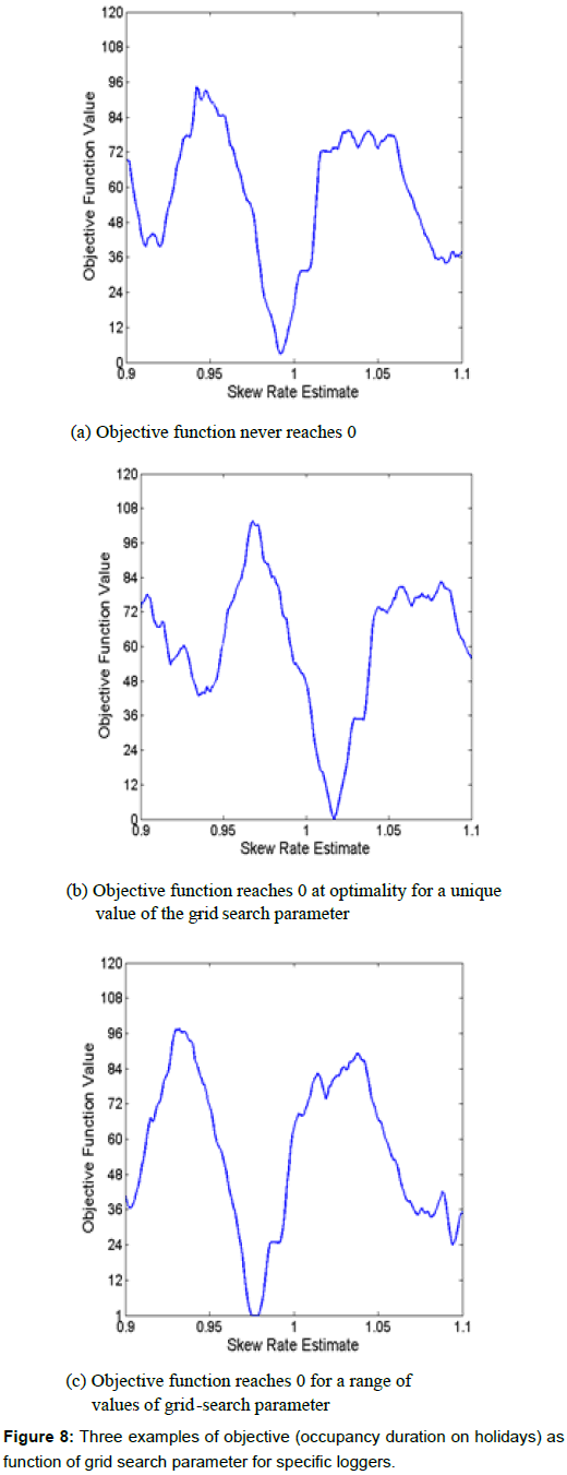
This is a single variable continuous optimization problem that has a very complicated objective function (as shown in Figures 8a, 8b and 8c, for three representative loggers). Also, we need to solve it only approximately because a more accurate estimation will follow in the subsequent step. Therefore, we opt for a simple grid search technique. Based on our prior knowledge about the accuracy of the clocks, we expected the skew rate to be at most 15 to 30 minutes per day, i.e., approximately 1%-2%. So, in order to be very conservative, we decided to focus our grid-search for the skew rate variable within the range of [0.9, 1.1]. Also, we decided to use 200 points in our grid. That way we fixed our tolerance value at 0.2/200=0.1%. Thus over a span of 100 days we are within approximately 2.5 hours error. This easily suffices the purpose of day-identification as specified for this task.
Figures 8a, 8b and 8c provide three different examples of the value of objective as a function of the grid-search parameter  . In the case of Figure 8a, the optimal objective function value does not reach 0 for any value of skew, but in Figure 8b there is a unique skew value at which the objective function dips to zero, while in Figure 8c, not only does the objective function value reach 0 at optimality, but it stays at zero for a range of skew rate estimates.
In order to avoid inclusion of false positive occupancy events, we excluded all occupancy periods of duration less than 20 minutes (as recorded by the logger) from this grid-search algorithm.
At the end of day-of-week estimation step, we have an approximate estimate of the clock skew, but it needs to be further refined, because:
1. We have just one skew-rate estimate for occupied and unoccupied times.
2. Even if the grid-search picks up the grid point which is the nearest to the actual skew rate, we would still have up to a maximum of 2.5 hours of error in the corrected time values.
3. In cases, where we have multiple optimal points identified in the grid search, estimation accuracy will be further impacted. For these cases, in the grid-search we arbitrarily decided to pick the lowest skew estimate that gives the zero objective function value in the grid-search.
Therefore, we proceed to the next step, which corresponds to the preprocessing step for the subsequent regression step.
Regression preprocessing
There are two main sub-steps within the regression preprocessing step, namely, a) identification of working-day blocks and b) assignment of each block to a day.
Identification of working-day blocks: As mentioned before, the raw data contains a sequence of timestamps each providing the illuminance value and the occupancy level at a particular point of time. A quick look at the data shows that, as one might expect, for various reasons people in office buildings often go in and out of rooms and other office spaces. Therefore, even during the time when an employee is at work (during working hours), the occupancy sensor might indicate several periods of occupancy and non-occupancy interspersed with each other. An example of a typical occupancy pattern might include a 2 hour occupied period, then a 40 minute unoccupied period, then a 10 minute occupied period, then a 45 minute unoccupied period, then a 3 hour 20 minutes occupied period and so on. At the end of the work day, one expects a sustained period of several hours (e.g. 8 to 15 hours) when the room is continuously unoccupied. But even that is often disturbed by short periods where maintenance personnel occupy the space or by false triggers indicating short occupancy periods, etc. So, in general, it can be a difficult task to identify workday start and end times from a given occupancy time series dataset. Therefore, we invested a significant amount of effort to identify good heuristic rules to identify the data entries corresponding to the start and end times of a working day, which can be used as inputs to the subsequent regression model.
The following rule-set was used for this purpose. Note that, in the following rule-set, the terms such as ShortOccupancyTimeRemovalThreshold, MinOutOfOfficeTimeBetweenBlocks, MaxBlockLengthThreshold, MinTotalOccupancyTimeInABlock and MinContinuousOccupancyTimeInABlock are parameters of the algorithm. The purpose of these rules was to identify sets of consecutive data entries such that each set is to be considered as belonging to the same working day block.
α. First, any occupied time period less than ShortOccupancyTimeRemovalThreshold minutes in length was excluded from the calculations involving identification of working-day block, i.e., that period was assumed to be unoccupied instead. This is done in order to remove false occupancy triggers.
β. Next, any two subsequent blocks have to be separated by at least MinOutOfOfficeTimeBetweenBlocks hours. If not, they will be considered the same block. This is done to ensure that a brief period for which a person steps out of the office during the day is not falsely assumed to be the end of his/her working day.
χ. Next, any block of length greater than MaxBlockLengthThreshold hours was excluded from the calculations involving identification of working-day block. This is done to ensure that the algorithm does not wrongly consider a sequence of data entries longer than a reasonable length (e.g. 18 hours) as a valid block.
δ. Next, a block with less than MinTotalOccupancyTimeInABlock minutes of total occupied time was be excluded from the set of observations. This ensures that the algorithms does not consider extremely short sequences of data entries (e.g., shorter than 150 minutes) as valid blocks.
ε. Next, a block without any continuous occupied time period of MinContinuousOccupancyTimeInABlock minutes or longer was excluded from the set of observations. This is done because a person in office, at some point of time, is assumed to be spending at least one block of continuous time (e.g. at least 1 hour) in his/her office.
We used the following values of these five parameters:
ShortOccupancyTimeRemovalThreshold=30
MinOutOfOfficeTimeBetweenBlocks=10
MaxBlockLengthThreshold=18
MinTotalOccupancyTimeInABlock=150
MinContinuousOccupancyTimeInABlock=60.
We chose the values listed above using our understanding of a typical work-day at the customer site and using a trial-and-error approach. But these values cannot be considered to be appropriate for all settings. In general, these parameters must be learned from the available data and based on any insights into typical work patterns at the targeted office location. Also a sensitivity analysis needs to be conducted to identify the impact of varying these parameter values on the estimation accuracy. The dependence of the estimation procedure on these five parameters (sensitivity analysis) is detailed in Subsection 6.1.
Assignment of each block to an actual day
Once working-day blocks have been identified, the data entries corresponding to the start and end times of all blocks are obtained and the correction based on estimated clock skew rate from the gridsearch algorithm is applied to these start and end times. After applying this correction, if the start and end times correspond to the same day (e.g. fall between 00:00-23:59 hours of the same day), then the block is assigned to that day. However, if they belong to different days, then that block is assigned to the day which contains the largest portion of that block.
Regression analysis
There are two main steps in the regression analysis phase, namely, a) logger-specific preliminary regression and outlier removal and b) cross-logger regression and accommodation of day-specific parameters. We describe these two steps below.
Logger-specific preliminary regression and outlier removal: In this step, we first perform a preliminary regression for each logger to estimate the parameters in equations (7) and (8) while excluding the day-specific additive bias ( pd , qd ) in workday start and end times and exclude personal additive bias rn in workday start times. Day-specific additive bias parameters are excluded simply because they cannot be estimated using data from just one logger, because the model is overspecified. Also, we would like to avoid having to estimate personal additive bias for both workday start and end times because that led to model instability in many cases. Note that we know apriori that our estimated bias values an,occ and an,unocc must lie in a small band around 1.0, which is ensured by fixing the workday start time parameter to zero. We choose to keep workday end time bias parameter rather than start time bias parameter in our estimated model based on our own observations that typically people tend to have more variation in the time at which they leave office in the evening than the time when they arrive at the office in the morning.
Thus, we estimate the parameters of the following equations for each logger n.
 (9)
(9)
and
 (10)
(10)
We estimate three parameters for each logger, namely and an,occ, an,unocc and sn. We used ordinary least squares estimator for this task.
After regressing first time, we identify and eliminate up to two outliers per logger. An observation is considered an outlier if the ratio of root-mean-squared error after and before removal is less than a certain threshold. We picked this threshold to be equal to the 4th power of the ratio of number of observations before and after removal. In general, the decision of what constitutes an outlier should be based on the improvement in some error measure and that needs to be weighed against the reduction in number of available observations due to outlier removal. Root mean squared error is chosen because it is consistent with the objective to be minimized in ordinary least squares regression analysis. Similar to the five parameters described in Sub-section 5.2, the choice of maximum number of outliers (MaxOutliers=2 in our case) and the power to which the ratio of number of observations is raised in order to compare with the ratio of root mean squared errors (PowerInOutlierRemoval=4.0 in our case) are both considered to be additional parameters to which the sensitivity of our results is tested. The results of the sensitivity analysis are described in Sub-section 6.1. Thus, these two additional parameters for which the sensitivity of our results is measured are:
MaxOutliers=2
PowerInOutlierRemoval=4
Additionally, the typical start and end times of a day (i.e.,  and
and  ) are assumed to be 8 am and 5 pm respectively (that is, TypicalDayStartTime=8 and TypicalDayEndTime=5). We also perform an analysis of the sensitivity of our results to these two parameters in Sub-section 6.1. Thus, these two additional parameters for which the sensitivity of our results is measured are:
TypicalDayStartTime=8
TypicalDayEndTime=5
Cross-logger regression and accommodation of day-specific constants
In this step, we first run a regression across loggers using the same model as given by equations (9) and (10). Next we identify the special days for which it makes sense to use a day-specific additive bias term for either the work-day start time or for the work-day end time, or for both. We avoid using an additive bias term for each day in order to keep the model simple and to avoid over-fitting. Note that, as mentioned earlier, if we use day-specific constants for all days, then the number of coefficients to be estimated will be increased by 50*2=100. We base the decision of whether to use an additive bias for a specific work-day’s start or end time based simply on whether the mean error for that day’s start or end time in the aforementioned first cross-logger regression run exceeds some threshold. This threshold (SpecialDayConstantThreshold) is yet another parameter for which the sensitivity analysis is performed. We use a default value of 1.5 hours for this parameter. That is,
SpecialDayConstantThreshold=1.5
After including these day-specific additive biases for start and/or end times of certain days, we estimate the final cross-logger regression model whose specification looks the same as equations (7) and (8) except that, pd and qd terms are included only for some selected days and the personspecific additive bias for the start time of a work-day (rn ) is set to zero for reasons mentioned earlier.
The results presented in Section 6 are obtained by using this final regression model.
Results and Discussion
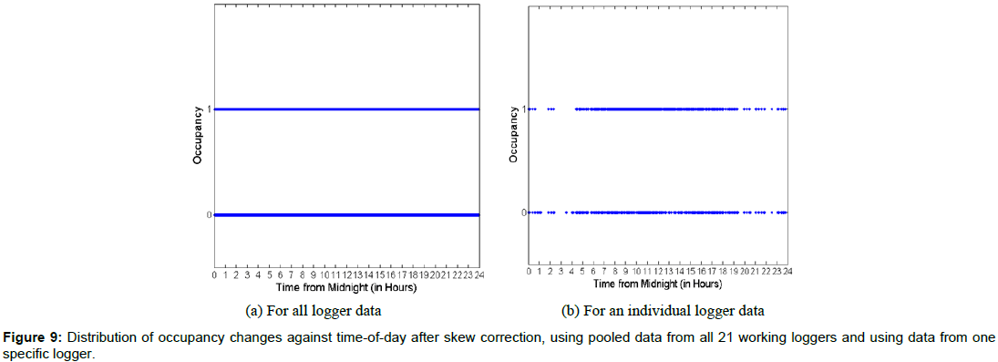
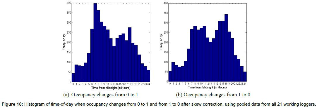
This section details the main results of our estimation process. We compare and contrast these results with the charts in Sub-section 4.1 which were generated using the raw data prior to skew correction. Figure 9a shows the distribution of occupancy changes against time-ofday using skew-corrected data and Figure 1b shows the corresponding distribution of occupancy changes against time-of-day using raw data prior to skew correction. Figure 9a shows the plot of occupancy against time-of-day for all 21 loggers, which fails to show any useful visual information due to too many data-points, similar to what is displayed in Figure 1b and Figures 10a, 10b show the distribution of times when occupancy changes from 0 to 1 and from 1 to 0 respectively, against timeof- day for the skew-corrected data. These two figures clearly indicate that a majority of 0-1 and 1-0 occupancy changes happen during 6 am and 9 pm for the skew-corrected data, in contrast to Figures 2a, 2b, which display almost uniform distribution of occupancy change times. Furthermore, Figure 10a shows that the 0-1 occupancy changes happen most often during the 7:00 am-10:00 am period which is a reasonable time period for many employees to enter their office in the morning. On the other hand, Figure 10b shows that the 1-0 occupancy changes happen most often during the 4:00-7:00 pm time period, which seems to be a reasonable time period for many employees to leave their office to go home in the evening. It is also interesting to note that there seems to be a quite a drop in the number of occupancy changes (both from 0 to 1 and from 1 to 0) during noon to 3:00 pm time period, which could possibly be because it includes most employee’s lunch times.
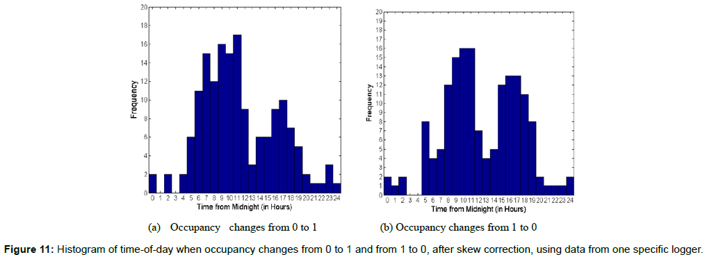
Figures 9b and 11a, 11b are analogous to Figures 9a and 10a, 10b respectively, but represent data for a specific logger rather than the data from all 21 loggers. Figure 9b shows that most occupancy changes happen during 6 am and 7:30 pm time period for this specific room after skew correction is applied, in contrast to the almost arbitrary distribution of occupancy change times before skew correction, as displayed by Figure 3b. Similarly, the trends in 0-1 and 1-0 occupancy changes for this specific logger as reflected in Figures 11a and 11b are similar to those for the entire 21-logger data as reflected in Figures 10a and 10b. This is in contrast with the lack of reasonable trends as displayed for pre-correction data in Figures 4a and 4b respectively.
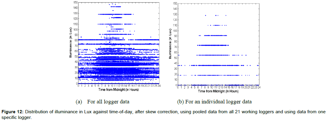
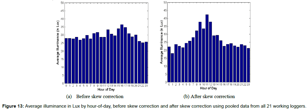
Figures 12a and 12b display the distribution of illuminance against time-of-day respectively for all loggers and for data from a specific logger. They are to be contrasted against Figures 1a and 3a respectively. As displayed in both Figures 12a and 12b, the illuminance is substantially higher during the 6:00 am to 6:00 pm time period. Such trends are absent in Figures 1a and 3a. Another way to visualize the data in Figures 1a and 12a is provided by Figures 13a and 13b respectively. These two figures show, for the pooled data from all 21 working loggers, the average illuminance for each hour of the day before and after skew correction respectively. Before skew correction, the average illuminance profile per hour looks very flat, whereas after skew correction, there is a clear peak around 11 am-noon time. Also, high average illuminance values are found for each hour between 6 am and 4 pm. All of this illuminance-related evidence displayed in Figures 12a, 12b, 13a and 13b, provides an independent validation of our skewcorrection algorithm, which does not use illuminance data at any step of the process. Intuitively, one expects the illuminance due to both natural and artificial lights to be higher during the working day than during the night time. The evidence in Figures 1a, 3a, 12a, 12b, 13a, 13b clearly demonstrates that the data after clock skew correction corroborates to this claim much more strongly than before the correction.
The results based on the pooled data from all 21 working loggers, which are graphically illustrated in Figures 1, 2, 9a, 10, 12a and 13, are succinctly summarized in Table 2. We divide each day into two periods. In the top three rows (excluding the header rows) of Table 2, we provide the percentage of occupancy changes that happen during the 7 am-7 pm period across all rooms with loggers, compared with the percentage of occupancy changes during the remaining 12 hours of the day. First row shows the 0-to-1 occupancy changes, second row shows the 1-to-0 occupancy changes and third row shows the combined total number of occupancy changes. For each row, we show the percentage occupancy changes before and after skew correction for the 7 am-7 pm period and for the 7 pm-7 am period. Additionally, in the fourth row after the header rows, we provide the average illuminance (in Lux) for the 7 am-7 pm period and for the 7 pm-7 am period for both the raw data and the skew-corrected data. For a significant part of the period between 7 am and 7 pm most people are expected to be in their workplaces and hence more frequent occupancy changes and higher average illuminance values are expected during that period. That is exactly what is observed in Table 2.
| Before skew correction | After skew correction | |||
|---|---|---|---|---|
| 7am-7pm | 7pm-7am | 7am-7pm | 7pm-7am | |
| Percentage of 0-1 occupancy changes | 47.60% | 52.40% | 68.50% | 31.50% |
| Percentage of 1-0 occupancy changes | 45.80% | 54.20% | 65.20% | 34.80% |
| Percentage of All occupancy changes | 46.70% | 53.30% | 66.90% | 33.10% |
| Average illuminance | 30.8 | 27.5 | 31.7 | 22.9 |
| 9am-3pm | 3pm-9am | 9am-3pm | 3pm-9am | |
| Average illuminance | 29.9 | 28.8 | 35.4 | 24.6 |
Table 2: Occupancy changes and higher average illuminance values.
Note that for the winter months of December through February for which the study was conducted, the sunrise times in U.K. can be late as (or even later than) 8 am. Similarly, the sunset times in U.K. during this period can be earlier than 4 pm. Therefore, the illuminance is expected to be especially higher during the six-hour period between 9 am and 3 pm every day. We test this hypothesis in the last row of Table 2 where we provide the average illuminance values (in Lux) for the 9 am-3 pm period and for the 3 pm-9 am period for both raw and skew-corrected data. The post-correction data clearly shows that the average illuminance is significantly higher in the 9 am-3 pm period than in the 3 pm-9 am period. However, such difference is not observed in the raw data. As noted earlier, this illuminance data was never used anywhere in the skew correction process, further validating our methodology and results.
Sensitivity analysis
As mentioned in Section 5, there are a number of parameters whose assumed values impact the performance of our overall algorithm for clock skew estimation. These parameters and their assumed values (also called base values from here onward) are the following.
1) ShortOccupancyTimeRemovalThreshold=30
2) MinOutOfOfficeTimeBetweenBlocks=10
3) MaxBlockLengthThreshold=18
4) MinTotalOccupancyTimeInABlock=150
5) MinContinuousOccupancyTimeInABlock=60
6) MaxOutliers=2
7) PowerInOutlierRemoval=4
8) TypicalDayStartTime=8
9) TypicalDayEndTime=5
10) SpecialDayConstantThreshold=1.5.
In addition to these 10, we also tested the sensitivity of the results to one more factor. Before using the day-of-week identification algorithm, we do some data preprocessing to ensure that we filter out any data that might indicate false positives recorded by the occupancy sensors. In some cases, very short occupancy intervals are noted by the sensor, which often occur because an instance of motion is followed by a timeoff delay interval without any motion. This results in small periods which are recorded as occupied times but often are equal to or slightly longer than the time-off delay period of the occupancy sensor. So in data cleaning, we try to remove these very short occupancy periods with length below a certain threshold. Let us denote this threshold by DataCleaningMinOccupancyTimeThreshold. It is measured in minutes. The default (base) value of this parameter that we used was DataCleaningMinOccupancyTimeThreshold=20.
We use the following four metrics to characterize the sensitivity of our results to these 11 parameters.
1. Number of observations available for the final cross-logger regression (NOBS): We use this measure to characterize the performance of the overall algorithm because, among other things, greater number of observations is beneficial for the stability and robustness of our results.
2. Root Mean Squared Error in the block start and end Times (RMSET): This measure characterizes the magnitude of remaining variations in the start and end times of workday blocks. This is measured in number of hours.
3. Sum of Squared Deviations in Clock Skews (SSDCS): This is defined as the sum of squares of differences between the clock skew values (both for occupied and unoccupied time periods) for each logger as compared to those for the base values ( b0n,unoccand b0n,unocc respectively). This gives a measure of how much the estimated skew values vary with variations in assumed parameter values.

4. Sum of Squared Clock Skew Percentage (SSCSP): This is defined as the sum of squares of percentage skews during occupied and unoccupied times for each of the loggers, where percentage skew is defined as the multiplicative factor that modifies the time measured by each logger minus 1. This gives us a measure of the magnitude of estimated clock skew.
 .
.
The variation in the values of each of these four metrics with variations in each of the 11 parameters listed above is given in Table 3. The first column of the table indicates the parameter that we varied to obtain the results in that row. Note that all the other parameters are kept at their base values for the results presented in that row. The second column indicates the new value of the parameter that is varied. The third column indicates the base value. Fourth through seventh columns indicate the values of the four metrics as described above, which are used to measure the sensitivity of the results. The first row below the header row indicates the metrics corresponding to the base values of all parameters. For each parameter, the row corresponding to the base value of that parameter is indicated in bold letters.
| Parameter | Value | Base | NOBS | RMSET | SSDCS | SSCSP |
|---|---|---|---|---|---|---|
| All base parameters | 826 | 1.9081 | 0 | 0.0377 | ||
| ShortOccupancyTimeRemovalThreshold ShortOccupancyTimeRemovalThreshold ShortOccupancyTimeRemovalThreshold ShortOccupancyTimeRemovalThreshold ShortOccupancyTimeRemovalThreshold ShortOccupancyTimeRemovalThreshold ShortOccupancyTimeRemovalThreshold |
15 20 25 30 35 40 45 |
30 30 30 30 30 30 30 |
709 798 817 826 816 824 819 |
2.0127 1.959 1.9486 1.9081 1.9348 1.992 1.9498 |
0.0085 0.0025 0.0007 0 0.0005 0.0022 0.0011 |
0.0412 0.0328 0.0347 0.0377 0.04 0.0474 0.0451 |
| MinOutOfOfficeTimeBetweenBlocks MinOutOfOfficeTimeBetweenBlocks MinOutOfOfficeTimeBetweenBlocks MinOutOfOfficeTimeBetweenBlocks MinOutOfOfficeTimeBetweenBlocks MinOutOfOfficeTimeBetweenBlocks MinOutOfOfficeTimeBetweenBlocks |
8.5 9 9.5 10 10.5 11 11.5 |
10 10 10 10 10 10 10 |
849 845 838 826 809 797 756 |
1.922 1.9213 1.9231 1.9081 1.9438 1.9899 2.0121 |
0.0001 0.0001 0 0 0 0.0003 0.0013 |
0.0368 0.0369 0.0375 0.0377 0.0375 0.0388 0.0409 |
| MaxBlockLengthThreshold MaxBlockLengthThreshold MaxBlockLengthThreshold MaxBlockLengthThreshold MaxBlockLengthThreshold MaxBlockLengthThreshold MaxBlockLengthThreshold |
15 16 17 18 19 20 21 |
18 18 18 18 18 18 18 |
820 822 823 826 827 827 827 |
1.8939 1.8933 1.8892 1.9081 1.9126 1.9126 1.9126 |
0 0 0 0 0.0001 0.0001 0.0001 |
0.0378 0.0376 0.0375 0.0377 0.038 0.038 0.038 |
| MinTotalOccupancyTimeInABlock MinTotalOccupancyTimeInABlock MinTotalOccupancyTimeInABlock MinTotalOccupancyTimeInABlock MinTotalOccupancyTimeInABlock MinTotalOccupancyTimeInABlock MinTotalOccupancyTimeInABlock |
60 90 120 150 180 210 240 |
150 150 150 150 150 150 150 |
853 851 834 826 802 792 787 |
1.9888 1.9896 1.9739 1.9081 1.895 1.9003 1.8784 |
0.0008 0.0007 0.0003 0 0.0051 0.0022 0.0027 |
0.0338 0.0339 0.0374 0.0377 0.0576 0.0494 0.0502 |
| MinContinuousOccupancyTimeInABlock MinContinuousOccupancyTimeInABlock MinContinuousOccupancyTimeInABlock MinContinuousOccupancyTimeInABlock MinContinuousOccupancyTimeInABlock MinContinuousOccupancyTimeInABlock MinContinuousOccupancyTimeInABlock |
30 40 50 60 70 80 90 |
60 60 60 60 60 60 60 |
830 830 830 826 817 808 790 |
1.9067 1.9067 1.9067 1.9081 1.9027 1.8933 1.9224 |
0.0001 0.0001 0.0001 0 0.0014 0.0017 0.0029 |
0.0361 0.0361 0.0361 0.0377 0.0468 0.0487 0.0539 |
| MaxOutliers MaxOutliers MaxOutliers MaxOutliers MaxOutliers MaxOutliers MaxOutliers |
0 1 2 3 4 5 6 |
2 2 2 2 2 2 2 |
846 838 826 823 821 821 821 |
2.1648 2.124 1.9081 1.9054 1.8984 1.8984 1.8984 |
0.0003 0.0001 0 0 0 0 0 |
0.0387 0.0364 0.0377 0.0379 0.0379 0.0379 0.0379 |
| PowerInOutlierRemoval PowerInOutlierRemoval PowerInOutlierRemoval PowerInOutlierRemoval PowerInOutlierRemoval PowerInOutlierRemoval PowerInOutlierRemoval |
2.5 3 3.5 4 4.5 5 5.5 |
4 4 4 4 4 4 4 |
811 815 820 826 830 832 833 |
1.7615 1.8411 1.8552 1.9081 1.9191 1.9198 1.9242 |
0.0006 0.0006 0.0006 0 0.0001 0.0001 0.0002 |
0.0392 0.0393 0.0393 0.0377 0.0401 0.0395 0.0395 |
| TypicalDayStartTime TypicalDayStartTime TypicalDayStartTime TypicalDayStartTime TypicalDayStartTime TypicalDayStartTime TypicalDayStartTime |
6.5 7 7.5 8 8.5 9 9.5 |
8 8 8 8 8 8 8 |
827 826 826 826 826 826 826 |
1.9134 1.919 1.9135 1.9081 1.9186 1.9131 1.9076 |
0.0001 0 0 0 0 0 0.0001 |
0.04 0.0395 0.0386 0.0377 0.037 0.0361 0.0353 |
| TypicalDayEndTime TypicalDayEndTime TypicalDayEndTime TypicalDayEndTime TypicalDayEndTime TypicalDayEndTime TypicalDayEndTime |
3.5 4 4.5 5 5.5 6 6.5 |
5 5 5 5 5 5 5 |
826 826 826 826 826 826 826 |
1.9081 1.9081 1.9081 1.9081 1.9081 1.9081 1.9081 |
0 0 0 0 0 0 0 |
0.0377 0.0377 0.0377 0.0377 0.0377 0.0377 0.0377 |
| SpecialDayConstantThreshold SpecialDayConstantThreshold SpecialDayConstantThreshold SpecialDayConstantThreshold SpecialDayConstantThreshold SpecialDayConstantThreshold SpecialDayConstantThreshold |
0.75 1 1.25 1.5 1.75 2 2.25 |
1.5 1.5 1.5 1.5 1.5 1.5 1.5 |
826 826 826 826 826 826 826 |
1.7996 1.8434 1.8669 1.9081 1.9576 1.9937 1.9937 |
0 0 0 0 0.0001 0.0001 0.0001 |
0.0368 0.0377 0.038 0.0377 0.0395 0.0396 0.0396 |
| DataCleaningMinOccupancyTimeThreshold DataCleaningMinOccupancyTimeThreshold DataCleaningMinOccupancyTimeThreshold DataCleaningMinOccupancyTimeThreshold DataCleaningMinOccupancyTimeThreshold DataCleaningMinOccupancyTimeThreshold DataCleaningMinOccupancyTimeThreshold |
5 10 15 20 25 30 35 |
20 20 20 20 20 20 20 |
824 824 826 826 826 826 816 |
2.2203 2.2203 1.9081 1.9081 1.9081 1.9081 1.9348 |
0.0082 0.0082 0 0 0 0 0.0005 |
0.0475 0.0475 0.0377 0.0377 0.0377 0.0377 0.04 |
Table 3: Sensitivity analysis.
In order to implement our algorithm as software accompanying the OccuSwitch data logger hardware, we need to ensure that the results are robust to individual parameter values that we assumed. Below is the summary of our findings about the sensitivity of the results.
• Sensitivity to ShortOccupancyTimeRemovalThreshold parameter: With any variations in this parameter above the value of 15 minutes, the estimated clock skew values do not vary much with the highest SSDCS values being 0.0025, which means that the root mean squared (RMS) deviation (0.0025/42) is about 0.77% translating into 11 minutes per 24 hours or 19 hours over a 100 day time period. The sum of squared clock skew percentages (SSCSP values) varies only between 0.0328 and 0.0474 over the entire range (of 15 through 45 minutes) of ShortOccupancyTimeRemovalThreshold values, which translates into RMS skew values in the range of 67 to 81 hours over 100 days. This displays relatively stable behavior compared to the estimated value of about 72 hours per 100 days. Most importantly, the root mean squared error in block start and end times (RMSET) varies only mildly between 1.9081 and 2.0127 (only about 5% variation). Notably, our base parameter value of ShortOccupancyTimeRemovalThreshold=30 minutes turns out to be the value that minimizes the RMSET value. The number of observations (NOBS) varies between 709 and 826, with the maximum NOBS value also corresponding to the base parameter value that we chose. Thus our choice of base value for the ShortOccupancyTimeRemovalThreshold parameter, which was originally based on a trial-and-error procedure, is further justified by this sensitivity analysis. This sensitivity analysis demonstrates that the choice of this parameter’s value can impact the SSDCS and SSCSP values to some extent but the impact on error (RMSET) is relatively low.
• Sensitivity to MinOutOfOfficeTimeBetweenBlocksparameter: As expected, the increasing value of this parameter translates to fewer observations being included in the regression analysis and therefore the NOBS value shows nondecreasing trend against this parameter value. For all values of MinOutOfOfficeTimeBetweenBlocksparameter below 11.5 hours, the clock skews are almost unaffected by variation in this parameter as can be seen from negligible SSDCS values and very stable SSCSP values. For MinOutOfOfficeTimeBetweenBlocks=11.5 hours, there is a slightly higher movement of SSDCS and SSCSP, but it is still small in an absolute sense. Once again, the RMSET value varies in a very thin band of 5.5% or so and the chosen parameter value turns out to be the one that minimizes RMSET. In summary, the sensitivity of our results to variations in this parameter is negligible.
• Sensitivity to MaxBlockLengthThreshold parameter: The impact of this parameter on all the four metrics, that is, NOBS, RMSET, SSDCS and SSCSP is very negligible. There is a small increase in the number of observations available for regression (from 620 to 627) with an increase in the value of this parameter, which is exactly as we intuitively expect. Also, with this increase in the number of observations, the accuracy decreases slightly as reflected by the trend in the RMSET values, which is again intuitively reasonable. In summary, we conclude that in the tested range, between 15 and 21 hours, our results are largely unaffected by the variation in this parameter.
• Sensitivity to MinTotalOccupancyTimeInABlock parameter: As one would expect, with an increase in this parameter’s value, the NOBS decreases. The accuracy, as reflected by the RMSET values, varies in a narrow 5% band between 1.8784 and 1.9888 around the base value of 1.9081. The SSDCS and SSCSP values are very stable up to 150 minutes. For parameter values greater than that the SSDCS and SSCSP values are a lot more dependent on this parameter’s value. In summary, the RMSET value is quite insensitive to the variations in this parameter’s value. The values of estimated skews are insensitive up to a certain point above which they become more sensitive. So it is best to restrict the chosen value of this parameter up to 150 minutes or so for stable results.
• Sensitivity to MinContinuousOccupancyTimeInABlock parameter: Including and below 60 minutes, the results (in terms of NOBS, RMSET, SSDCS and SSCSP values) are highly insensitive to this parameter. However, with increasing value of this parameter, the results become more sensitive, presumably because large occupied periods get omitted, which starts resulting in some drop in NOBS and decrease in accuracy. Also, the NOBS value drops with increase in this parameter, which is exactly what we expect intuitively. In summary, the value of this parameter should not be increased beyond a certain threshold (say 80 minutes or so); the base value seems quite reasonable; and results are insensitive to variation is this parameter within a small band above and a large band below this base value.
• Sensitivity to MaxOutliers parameter: With an increase in this parameter, the estimation error (RMSET) drops up to a certain point and becomes stable from there onwards. As more outliers are removed the error improves and the number of observations drops. However, the results are extremely insensitive to this parameter beyond MaxOutliers=2. Furthermore, even below this value, the results are only slightly sensitive to the changes in this parameter’s value. This also justifies our choice of parameter.
• Sensitivity to PowerInOutlierRemoval parameter: As one would expect, with an increase in this parameter’s value, NOBS value increases. The error (RMSET) remains largely unaffected. There is also not a significant dependence of the SSDCS and SSCSP values on the value of this parameter. Furthermore, the base value of this parameter results in the lowest possible value of SSCSP in this range. This also justifies our choice of base parameter value.
• Sensitivity to TypicalDayStartTime parameter: As seen in Table 3, the impact of this parameter on NOBS, RMSET and SSDCS is zero or negligible. SSCSP has a clear decreasing trend indicating that the net skew in clocks is negative (i.e., roughly speaking, more clocks are slower than faster). With this parameter varying over three hours (6:30 am to 9:30 am) the corresponding variation in SSCSP is equivalent to 4.5 hours over 100 days or 2.7 hours over 60 days. These numbers make a lot of sense intuitively, especially given the fact that we have a special factor for adjusting each logger’s block end times in our regression model. In summary, all variations in results are either negligibly small, or intuitively reasonable, or both.
• Sensitivity to TypicalDayEndTime parameter: As can be seen in Table 3 this parameter, by construction, has no impact on any results. This is because of the structure of our regression model which has a special term (Sn) to adjust for this effect, as shown in equations (3) and (4).
• Sensitivity to SpecialDayConstantThreshold parameter: This parameter has zero impact on NOBS and a very negligible impact on the SSDCS values. There is a less than 4% variation in the value of SSCSP with variations in this parameter. The error, as one expects, increases with an increase in the value of this parameter.
• Sensitivity to DataCleaningMinOccupancyTimeThreshold parameter: These results clearly demonstrate the value of data cleaning efforts before beginning the actual estimation. As long as the value of this parameter is at least 15 minutes, the results are extremely insensitive to the value of this parameter. However, for DataCleaningMinOccupancyTimeThreshold=5 and 10 minutes, false positives in occupancy data cause a considerable decrease in error and the results do depend on this parameter value. This justifies the present choice of the base parameter value because the results are very insensitive to variations in this parameter within a band around the base value.
Conclusion
In this study, we proposed a low-power system for accurate logging of timestamp data on occupancy and light levels at individual customer sites. The system consists of OccuSwitch data loggers and accompanying software to analyze the logged data. The OccuSwitch data logger consists of a combination of two clocks, a high-power high-accuracy clock to measure timestamps when higher accuracy is warranted and a low-power low-accuracy clock to measure timestamps when greater power-efficiency is warranted. The low-power clock is used for a large proportion of the logging time period thus resulting in longer battery life for the data logger. However, the lower accuracy introduces a skew in timestamp measurements. In this study, we describe an analytical framework to model the clock skew by exploiting the cyclical nature of occupancy patterns in commercial buildings. The model is solved using a computational approach combining grid-search based optimization and regression algorithms. The results are validated against illuminance (light level) data. Our results show that our algorithm has a good accuracy level. We also conduct a sensitivity analysis indicating that the results are robust to small changes in parameter values. Additionally, the importance of good data cleaning heuristics is also illustrated by our results. Overall, our estimation, validation and sensitivity results demonstrate that accurate visualizations and energy saving estimates can be generated using our approach.
Acknowledgement
This research was performed at Philips research N.A. labs in Briarcliff Manor, NY. All three authors were Philips employees when this research was conducted.
References
- Audin L (1999) Occupancy sensors: Promises and pitfalls. Esource Tech Update, TU-93-8, Boulder CO.
- Garg V, Bansal NK (2000) Smart occupancy sensors to reduce energy consumption. Energy and Buildings 32: 81-87.
- Neida BV, Maniccia D, Tweed A (2001) An analysis of energy and cost savings potential of occupancy sensors for commercial lighting systems. J Illuminating Eng Soc 30: 111-125.
- Guo X, Tiller DK, Henze GP, Waters CE (2010) The performance of occupancy-based lighting control systems: A review. ‎Lighting Res Technol 42: 415-431.
- Dubois MC, Blomsterberg A (2011) Energy saving potential and strategies for electric lighting in future North European, low energy office buildings: A literature review. Energy and Buildings 43: 2572-2582.
- Leslie R, Raghavan R, Howlett O, Eaton C (2005) The potential of simplified concepts for daylight harvesting. Lighting Res Technol 37: 21-38.
- Galasiu AD, Newsham GR, Suvagau C, Sander DM (2007) Energy saving lighting control systems for open-plan offices: A field study. Leuko 4: 7-29
- Colaco SG, Kurian CP, George VI, Colaco AM (2008) Prospective techniques for effective daylight harvesting in commercial buildings by employing window glazing, dynamic shading devices and dimming control: A literature review. Building Simulation 1: 279-289.
- Sarkar A, Fairchild M, Salvaggio C (2008) Integrated daylight harvesting and occupancy detection using digital imaging. Proceedings of SPIE (The International Society for Optics and Photonics).
- Lu J, Birru D, Whitehouse K (2010) Using simple light sensors to achieve smart daylight harvesting. Proceedings of the Second ACM Workshop on Embedded Sensing Systems for Energy-Efficiency in Building 73-78.
- Neves-Silva R, Ruzzelli A, Fuhrmann P, Bourdeau M, Perez J, et al. (2010) Energy consumption prediction from usage data for decision support on investments: The EnPROVE approach. Control Methodologies and Technology for Energy Efficiency, Portugal.
- Parker D, Hoak D, Cummings J (2008) Pilot evaluation of energy savings from residential energy demand feedback devices. Florida Solar Energy Center, USA.
- Vieira R (2006) The energy policy pyramid-a hierarchal tool for decision makers. Fifteenth Symposium on Improving Building Systems in Hot and Humid Climates, Orlando, USA.
Citation: Vaze V, Patel M, Bagheri S (2017) A Data-Driven Approach for Accurate Estimation and Visualization of Energy Savings from Advanced Lighting Controls. Innov Ener Res 6: 177. DOI: 10.4172/2576-1463.1000177
Copyright: © 2017 Vaze V, et al. This is an open-access article distributed under the terms of the Creative Commons Attribution License, which permits unrestricted use, distribution, and reproduction in any medium, provided the original author and source are credited.
Select your language of interest to view the total content in your interested language
Share This Article
Recommended Journals
Open Access Journals
Article Tools
Article Usage
- Total views: 4683
- [From(publication date): 0-2017 - Nov 05, 2025]
- Breakdown by view type
- HTML page views: 3689
- PDF downloads: 994

