A Computational Dynamic Fluid Analysis of Compressible Flow in PorousMedia
Received: 23-Feb-2017 / Accepted Date: 17-Apr-2017 / Published Date: 24-Apr-2017 DOI: 10.4172/2576-1463.1000152
Abstract
The study is a computational dynamic analysis which investigated the dynamics of fluid flow patterns in a homogeneous oil reservoir using the Radial Diffusivity Equation (RDE). The model was solved analytically for pressure using the Constant Terminal Rate Solution (CTRS) and numerically using the fully implicit Finite Difference Method (FDM). Results from the study indicated that the initial reservoir pressure would be able to do the extraction of oil for an extended period of time before any other recovery method would be used to aid in further extraction process depending on the rate at which oil is produced. The study further confirmed that reservoir simulation describing a radial flow of a compressible fluid in porous media may be adequately performed using ordinary laptop computers. It could be seen from the analysis of the plots of pressure vs. time, and space that the Pressure Transient Analysis (PTA) was duly followed. The approximate solutions of the analytical and numerical solutions to the model were in excellent agreement, thus the reservoir simulation model developed could be used to describe typical pressure-time relationships. The analytical solution was used to verify the numerical solution as an application. Overall, this study provides an improved platform for modeling single phase flow in oil and gas reservoirs.
Keywords: Modeling; Simulation; Flow rate; Reservoir permeability; Viscosity; Compressible; Ghana
22616Introduction
Oil occurs in a natural state under pressure in underground rock formations in which it has accumulated over geologic time. Where the rock formations are porous and permeable, the natural resource may be exploited through wells drilled into the reservoirs. Oil reservoirs may be complex in nature, with physical properties that exhibit high degrees of anisotropy and heterogeneity.
The discovery of the Jubilee oil-fields offshore southwest Ghana is an asset in the economic development of Ghana. Indeed, due to the depletion of the currently exploited fields and the rarefaction of new field discovery, the Jubilee fields are going to open new economic opportunities for this country. However, the control of a rational exploitation of a field means mastering various scientific techniques including the understanding of the dynamics of fluids in place. During the exploitation, fluids can enter and replace the fluids already in position; phases can appear or disappear, etc. However, the physical phenomena involved in an oil reservoir are complex. The understanding of these phenomena requires then the combination of physics, mathematics and computing. Oil reservoir simulation serves an important role in forecasting oil production, understanding surface subsidence, predicting strain and stress development in the oil field, and preventing well damage [1]. Oil reservoirs are composed by porous media, which include both a solid phase and pore spaces filed with oil, gas and water. The pore pressure and the strain in the solid matrix have instant interaction between each other. Any change of the pore pressure or the depletion of fluid volume will affect the strain of the solid, or vice versa [1,2].
During the exploitation, fluids can enter and replace the fluids already in position; phases can appear or disappear, etc. However, the physical phenomena involved in an oil reservoir are complex. The understanding of these phenomena requires then the combination of physics, mathematics and computing [1]. The success of this technique is very dependent on the fluid flow pattern. Therefore, the numerical simulation of petroleum reservoir is of great importance in petroleum engineering, since full experimental simulation in laboratory is impossible.
The area under study is the site of the initial commercial oil and gas find, which is now known as Jubilee Field, and is located in the Tano and Cape Three Points Basins. It is estimated to hold oil reserves of between 800 million and 3 billion barrels, and substantial natural gas reserves.
Ghana has four sedimentary basins, the Voltaian Basin (Neo- Proterozoic, inland), Saltpond or Central Basin (Paleozoic, offshore), Accra-Keta or Eastern Basin (Cretaceous, offshore with onshore extension), and Tano-Cape Three Points or Western Basin (Cretaceous, offshore with onshore extension).
The Paleozoic and Cretaceous basins form Ghana’s continental margin, which stretches from the Ghana-Togo border in the east to the Ghana-Cote D’Ivoire border in the west [2]. The margin is part of the Gulf of Guinea Province. The Tano-Cape Three Points Basin is a Cretaceous wrench modified pull-apart basin bounded by the Saltpond Basin in the East and the St. Paul Fracture Zone in the West. The basin is the eastern extension of the Cote d’Ivoire-Ghana Basin and formed as a result of trans-tensional movement during the separation of Africa and South America, and the opening of the Atlantic Ocean in the Albian. Active rifting and subsidence during this period resulted in the formation of a deep basin [2].
Prevailing conditions at the time were ideal for the deposition of shales, thus thick organic rich shale was deposited in the Cenomanian and Turonian [3].
The Jubilee Fields, comprising Tano, Cape Three Point sub-basin in Ghana, which is part of the larger Ivory Coast Basin, located in the Gulf of Guinea, West Africa. It is located in about 75 m of water, 35 km offshore of Ghana. The location is about 4°46’ north latitude and about 3o west longitude. It is East-West onshore offshore structural basin [4].
Several river systems contributed significant clastics into the deep basin and led to deposition of large turbidite fan/channel complexes [5]. The working play type is the Cretaceous Play, which consists of Cenomanian-Turonian and Albian shales as source rocks with Turonian slope fan turbidite sandstones and Albian sandstones in tilted fault blocks as reservoirs. Trapping is both stratigraphic and structural [6].
The hydrocarbon potential of Ghana’s portion of the basin has been known since the 1890’s based on onshore oil seeps but the first major discovery was made in 2007 by Tallow Oil PLC (Jubilee Field) with oil production commencing in 2010. The hydrocarbon prospectively of the basin is also well known in Cote d’Ivoire where there are producing fields including Baobab, Belier, Espoir, Foxtrot, Lion and Panthere [7]. The Basin occupies an area of at least 3000 square kilometers in offshore and narrow onshore segment of the southwestern corner of the Republic of Ghana. It includes the narrow Mesozoic coastal strip of southwestern Ghana, the continental shelf, and steep submarine Ivory Coast Ghana ridge which form the continental slope [8].
The study of porous medium flow in reservoirs has its basis from Darcy’s law. Darcy’s law, describing a linear relationship between volumetric flow rate (Darcy’s velocity) and pressure (or potential) gradient, has been the fundamental principle in analysing flow processes in porous media. Any deviation from this linear relation maybe defined as non-Darcy flow and in most cases must first be linearized. In this study linearized Darcy’s law has been exclusively used.
The numerical solution of the proposed mathematical model is based on a discretization scheme. The final discretized equations are handled fully implicitly with the Finite Difference Method (FDM). As application example, the analytical solution is used to verify the numerical solution.
Model Formulation
The equations governing fluid flow in oil reservoirs are presented in this section. The models are one-dimensional, with variables resolved in the radial direction only. The equations for flow in porous materials were based on mass, momentum and energy conservation equations, and constitutive equations for the fluids and the porous material. For simplicity, isothermal conditions were assumed, so that energy conservation equation was replaced (However, in cases of changing reservoir temperature, such as in the case of cold water injection into a warmer reservoir, this may be of importance).
 (1)
(1)
The above equation (1) is the model for the radial flow of the single phase fluid in a porous medium. Equation (2) however the linearized form of equation (1), equation (3) on the other hand is the discretised form of the generalised model.
The equation was solved numerically by fully implicit (backward in time) finite difference scheme, where the system domain was treated as a set of mesh points and the pressure represented as nodal points.
The subscript i-1 and i+1 indicated position in the Finite Difference mesh and superscript n and n+1 denoted previous and current time levels respectively as shown in equation (3).
The cells designated i-1 and i+1 had the nodal pressures Pi+1, Pi and Pi-1
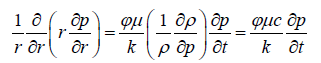 (2)
(2)
The above equation (2) was numerically approximated to:
 (3)
(3)
Where
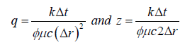 (4)
(4)
The space and time derivatives of the mathematical model were expressed as finite-difference terms in this section. Since the finite-difference equation was solved implicitly (4). All position subscripts and time-level superscripts will be consistent with the implicit method of solving a FDE. For implicit handling, the time derivative will be approximated by a standard backward difference, while the spatial difference is expressed at the unknown (n+1) time level. The physical model for the pressure analysis was discretized into grid points using space and time steps of 1 m and 1 h respectively (Tables 1 and 2) [9-14].
| Radial Distance (R)m | Analytical Model Pressure(pa)1.0e+06 | Numerical Model Pressure(pa)1.0e+06 |
|---|---|---|
| 1 | 8.273708787532529 | 8.273708785256742 |
| 2 | 8.273708817476488 | 8.273708815200701 |
| 3 | 8.273708834992581 | 8.273708832716793 |
| 4 | 8.273708847420446 | 8.273708845144659 |
| 5 | 8.273708857060248 | 8.273708854784459 |
| 6 | 8.273708864936539 | 8.273708862660751 |
| 7 | 8.273708871595849 | 8.273708869320060 |
| 8 | 8.273708877364404 | 8.273708875088618 |
| 9 | 8.273708787532529 | 8.273708880176844 |
| 10 | 8.273708817476488 | 8.273708884728420 |
Table 1: Pressure at different radial distances for analytical and numerical models.
| Time (Days) | Analytical Model Pressure(pa)1.0e+06 | Numerical Model Pressure(pa)1.0e+06 |
|---|---|---|
| 1 | 8.273708739468049 | 8.273708740340805 |
| 2 | 8.273708724496069 | 8.273708725368826 |
| 3 | 8.273708715738023 | 8.273708716610781 |
| 4 | 8.273708709524090 | 8.273708710396846 |
| 5 | 8.273708739468049 | 8.273708705576945 |
| 6 | 8.273708724496069 | 8.273708701638800 |
| 7 | 8.273708715738023 | 8.273708698309147 |
Table 2: Pressure at various times (t) for analytical and numerical models.
Results and Discussion
Results presented in the following figures were obtained by one dimensionally simulating the model, for transient flow. They show the evolution of the pressure during oil extraction, the figures show the distribution of pressure in the reservoir per day for seven days of production using the analytical method.
The transient flow which is most often modelled with the RDE, allows modelling pressure vs. time and pressure vs. radial distance from an observation point. The following section presents simulations that show pressure distributions across the various regions of the reservoir with time and space, and illustrate what is going on in the reservoir and to help understand the results of the analysis.
The analytical solution of the pressure distribution was made through investigations of an assortment of pressure vs. radius, and pressure vs. time plots for various producing times. Figures 1-3 illustrates the expected radial pressure distributions generated by the analytical model for production time of seven days. From Figure 1, it can be seen that on the first day of production, there is a sharp drop in pressure.

Figure 1: Flow region on radial coordinates for a period of seven days.

Figure 2: Flow region on square radial coordinates at different producing times for a period of seven days.

Figure 3: Flow region on inverse radial coordinates for a period of seven days.
It was however observed from the figures above that, radial distance within the reservoir increases with increasing pressure as fluid moves from the reservoir towards the wellbore. Figure 4 rather show decreasing pressure with decrease in radial distance. Figure 4 however illustrates the linear relationships expected between pressure and radius with logarithmic abscissa.

Figure 4: Flow region on logarithmic radial coordinates for seven days.
The pressure distributions shown by Figures 1-3 are typical of radial flow systems, showing large pressure gradients near the wellbore and smaller pressure gradients at locations further from the wellbore.
For the producing times considered, the pressure change at the external boundary of the model is negligible; therefore, the pressure distributions shown by Figures 1-3 are for the "infinite-acting" flow period.
This profile, shown in Figure 2, also reveals a variable pressure gradient, which is largest near the well. This important observation indicates that most of the pressure drop occurs near the production end of the system, a feature of radial flow that calls for considerable care when drilling and completing petroleum wells. This profile however shows a typical radial flow in oil reservoirs towards a well.
At a sufficiently large time, the pressure disturbance anywhere in the reservoir is proportional to the logarithm of the inverse square of the radius away from the origin of the disturbance. Thus, the magnitude of the disturbance is maximum near its origin (the wellbore) and rapidly terminates away from the wellbore.
Pressure is approximately a linear function of the logarithm of the radial distance during unsteady-state flow. The radius of influence of a pressure disturbance is also proportional to the square root of time.
The change in pressure Δp, and elapsed flow time Δt, as illustrated graphically in Figure 5 below, shows a classical reservoir pressure transient response. Plots of Δp versus Δt are important aspects of reservoir pressure analysis.

Figure 5: Flow region on time coordinates for different radial distances.
From the distributions below, the change in pressure across the entire region of the reservoir is not significant and therefore negligible for the given production period of seven days.
Figure 1 shows that at time t=1 day, the pressure disturbance has moved a distance r=1 m into the reservoir. Notice that the pressure disturbance radius is continuously increasing with time. This radius is commonly called the radius of investigation and referred to as rinv. It is also important to point out that as long as the radius of investigation has not reached the reservoir boundary, i.e., re, the reservoir will be acting as if it is infinite in size. During this time it could be said that the reservoir is infinite acting because the outer drainage radius re, can be mathematically infinite, i.e., re = ∞ . A similar discussion to the above can be used to describe a well that is producing at a constant bottom-hole flowing pressure.
Figure 4 also illustrates the propagation of the radius of investigation with respect to time. At time t=7 days, the pressure disturbance reaches the boundary. This causes the pressure behaviour to change. Based on the above discussion, the transient flow is defined as that time period during which the boundary has no effect on the pressure behaviour in the reservoir and the reservoir will behave as if it is infinite in size.
The transient flow period occurs during the time interval 0<t<1 and during the time period 0<t<7 for both constant flow rate and pressure scenario. The analytical and numerical solutions shown in Figures 1-15 also indicated that for a period of seven days the pressure in the reservoir was still enough to derive the oil towards the well for extraction, since the change in pressure from the initial reservoir pressure to the current reservoir pressure was almost negligible, thus the primary recovery method will be enough for production for the entire seven days of production period.

Figure 6: Flow region on logarithmic time coordinates for different radial distance.

Figure 7: Flow region on inverse time coordinates for different radial distance.

Figure 8: Flow region on square time coordinates for different radial distance.

Figure 9: Flow region on logarithmic square time for different radial distance.

Figure 10: Matlab graphing routine for the analytical solution for transient flow.

Figure 11: Comparison of pressure distributions of the analytical and numerical model.

Figure 12: Pressure distributions of the analytical and numerical models (RDE).

Figure 13: Pressure distributions of the analytical and numerical model (RDE).

Figure 14: Pressure distributions of the analytical and numerical model (RDE).

Figure 15: Pressure distributions of the numerical model for transient flow.
With the radial model being an ideal model, it is shown that the reservoir pressure is initially constant throughout, and the well is opened to flow at constant rate along its full wellbore thickness, the pressure transient moves out radially from each point in the wellbore with both time and space, as shown in the Figures above.
Near the wellbore, the pressure transient response, through the reservoir moves radially away from the well. This movement is rapid initially, but as it spreads out further from the wellbore and contacts progressively larger reservoir volume, it slows in its radial advance. Fluid movement takes place in those regions of the reservoir where the pressure has fallen below the original reservoir pressure.
Even though the production rate at the well is constant, the flux rate will be different at each radius because the cross-sectional area exposed to radial flow at each radius differs. The pressure response is a form of pressure transient, and the interpretation of it comprises one aspect of Pressure Transient Analysis (PTA).
The transient condition is only applicable for a relatively short period after some pressure disturbance has been created in the reservoir. In practical terms, if pressure is reduced at the wellbore, reservoir fluids will begin to flow near the vicinity of the well.
The pressure drop of the expanding fluid will provoke flow from further, undisturbed regions in the reservoir. The pressure disturbance and fluid movement will continue to propagate radially away from the wellbore.
The gradually extending region affected by flow is seen in Figures 1, 2 and 10. In the time for which the transient condition is applicable, it is assumed that the pressure response in the reservoir is not affected by the presence of the outer boundary, thus the reservoir appears infinite in extent.
Summary and Conclusion
This paper presents a general mathematical model and numerical approach to simulate single phase flow in porous media. Plot of both the analytical and numerical approaches are discussed in this paper. The use of reservoir simulation to describe Pressure Transient Analysis (PTA) has proved very successful. Simulation results with MATLAB have been compared with analytical results and the comparison showed that reservoir simulation can be used to investigate PTA in homogeneous oil reservoirs, specifically, oil reservoirs of the Jubilee Field, Tano Basin or reservoirs with the same physical properties. Through the course of developing the simulation model, programming the numerical methods, and studying the fluid dynamics and patterns in the reservoir, the model for studying the dynamics and patterns of fluid flow in oil reservoirs in homogeneous porous media was developed.
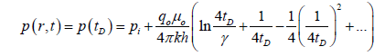
The model was solved analytically by the CTRS, with given initial and boundary conditions. The analytical solution was used to verify the numerical solution as an application example
Numerically the model was also solved using the fully implicit FDM to give the numerical solution of the pressure profile in the reservoir. The approximate solutions of the analytical and numerical solutions to the model were in excellent agreement, thus the reservoir simulation model developed can be used to describe typical pressure-time relationships that are used in conventional PTA.
It also adequately predicted that the initial reservoir pressure will be able to do the extraction for a very long time dependent on the rate of production, before any other recovery method will be used to aid in the extraction process. After successfully developing a model for the analysis of pressure distributions in oil reservoirs, further studies based on the results and findings of the work may lead to a better understanding of fluid flow patterns in oil reservoirs and other flow patterns that are not covered in the current study.
This study should be repeated without linearizing the flow equation so that results from that study could be compared to also the current study for further analysis.
Although excellent agreement between the analytical and numerical models has been achieved, the verification presented so far has been limited to one set of reservoir parameters. Therefore, the dimensionless forms of time (tD) and pressure (PD) should be developed and use to verify the model for a wide range of reservoir parameters. The verification of the model using dimensionless variables will be significant because it automatically verifies the numerical model for any assemblage of reservoir properties.
Acknowledgement
The authors wish to thank the Chinese Scholarship Council (CSC) for their tremendous support. The authors would also like to thank the following institutions, GNPC and the Petroleum Commission of Ghana.
References
- Ahamadi MEH, Rakotondramiarana HT (2014) Modeling and Simulation of Compressible Three-Phase Flows in an Oil Reservoir: Case Study of Tsimiroro Madagascar. Am J Fluid Dyn 4: 181-193.
- Atta-Peters D, Salami MB (2004) Late Cretaceous to early tertiary pollen grains from offshore Tano basin, Southwestern Ghana. Revista Espanola de Micropaleontologia 36: 451-465.
- Davies DW (1986) The Geology and Tectonic Framework of the Republic of Ghana and the Petroleum Geology of the Tano Basin. Southwestern Ghana. Internal Report, GNPC.
- Atta-Peters D, Kyorku NA (2013) Palynofacies analysis and sedimentary environment of Early Cretaceous sediments from Dixcove 4-2X well, Cape Three Points, Offshore Tano Basin, Western Ghana. Int Res J Geo Min 3: 270-281.
- Atta-Peters D, Garrey P (2014) Source rock evaluation and hydrocarbon potential in the Tano basin, South Western Ghana, West Africa. Int J Oil Gas Coal Eng 2: 66-77.
- Adda GW (2013) The Petroleum Geology and Prospectivity of the Neo-Proterozoic, Paleozoic and Cretaceous Sedimentary Basins in Ghana. Search and Discovery.
- Mah G (1987) Geological Evaluation of the onshore North Tano Basin. GNPC Internal Report.
- Dake LP (1978) Fundamentals of reservoir engineering, Amsterdam: Developments in petroleum science 8.
- Dake LP (1983) Fundamentals of reservoir engineering, Amsterdam: Developments in petroleum science.
- Dake LP (2001) The Practice of Reservoir Engineering Amsterdam: Developments in Petroleum Science 36.
- Dalen V (1979) Simplified finite-element models for reservoir flow problems. Soc Petrol Eng J 19: 333-343.
- Darcy H (1856) Flow of Water through sand filters for water purification.
- Odeh AS (1965) Unsteady-state behavior of naturally fractured reservoirs. Soc Petrol Eng J 5: 60-66.
Citation: Gawusu S, Zhang X, Solomon KP, Abdul-Wadud A (2017) A Computational Dynamic Fluid Analysis of Compressible Flow in Porous Media. Innov Ener Res 6: 152. DOI: 10.4172/2576-1463.1000152
Copyright: © 2017 Gawusu S, et al. This is an open-access article distributed under the terms of the Creative Commons Attribution License, which permits unrestricted use, distribution, and reproduction in any medium, provided the original author and source are credited.
Share This Article
Recommended Journals
Open Access Journals
Article Tools
Article Usage
- Total views: 5012
- [From(publication date): 0-2017 - Apr 02, 2025]
- Breakdown by view type
- HTML page views: 4054
- PDF downloads: 958